04 - Core Concepts

This chapter introduces the core concepts and workflow of LESS. After understanding these concepts, you will be able to flexibly combine various functions to complete complex remote sensing simulation tasks.

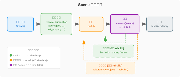
Scene lifecycle: build, simulate, and rebuild

LESS Scene is a persistent, reusable digital scene. Its structural-spectral separation architecture allows geometry and acceleration structures to be reused across simulations, while sensor bands, illumination, and properties are updated for each run.

import less

# 1. Create a scene
scene = less.Scene()
scene.size = 50.0

# 2. Configure scene elements
scene.terrain = less.Terrain(property=less.Lambertian(reflectance=0.15))
scene.illumination = less.Illumination(source=less.Sun(zenith=30, azimuth=150), atmosphere=less.NoAtmosphere())
tree = less.Object("ash", mesh=less.examples.asset_path("FREX.obj"))
tree.set_property("leaves", less.Prospect(cab=40))
tree.set_property("stem_branch", less.Lambertian(reflectance=0.1))

scene.add(tree, positions=[[25, 25, 0]])

# 3. Simulation → automatically build scenarios and obtain products when necessary
image = scene.simulate(less.OpticalImager(
    less.Orthographic(image_size=512),
    bands=[650, 550, 450],
))

# 4. Modify the parameters and simulate again (no rebuild required)
scene.illumination = less.Illumination(source=less.Sun(zenith=50, azimuth=200), atmosphere=less.NoAtmosphere())
image2 = scene.simulate(less.OpticalImager(
    less.Orthographic(image_size=512),
    bands=[650, 550, 450],
))

# 5. Image visualization
image.show() # Raw radiance visualization
image.to_brf().show() # Convert to BRF and then visualize

simulate(): the default entry for ordinary users

scene.simulate(...) can automatically build scenes. If the scene has not been built yet, LESS will automatically build it before the first simulation; subsequent simulations will reuse existing native scenes and acceleration structures as much as possible.

image = scene.simulate(sensor)

The sensor band will be re-prepared according to this simulation, so there is no need to call build() in advance to change the band.

build(): Optional explicit preparation step

build() is an optional explicit preparation step. It is used to verify the scene in advance, load geometry, upload resources and build an acceleration structure. For example, when it is necessary to measure the construction time and simulation time separately:

scene.build()
image = scene.simulate(sensor)

build() is idempotent: for a scene that has been built and has not changed, calling it again usually reuses the existing native scene instead of unconditionally rebuilding it. The dynamic instance interface Scene.update_instances() also requires that the scene has been explicitly constructed.

rebuild(): Force a complete rebuild

rebuild() is used to force a complete rebuild: it refreshes the native scene representation, rereads or uploads the geometry, and rebuilds the acceleration structure.

scene.rebuild()

A typical use is that an external program modifies the OBJ file under the same path, but LESS cannot determine from the path change that the file content has changed.

Modifying properties or lighting usually does not require calling rebuild():

scene.terrain.set_property(
    less.Lambertian(reflectance=0.2)
)
scene.illumination = less.Illumination(
    source=less.Sun(
        zenith=45,
        azimuth=scene.illumination.source.azimuth,
        spectrum=scene.illumination.source.spectrum,
        wavelengths=scene.illumination.source.wavelengths,
        irradiance=scene.illumination.source.irradiance,
    ),
    atmosphere=scene.illumination.atmosphere,
)

image = scene.simulate(sensor)

LESS will update relevant parameters and reuse existing geometry and BVH as much as possible. When the geometry is modified by exposing API, LESS will maintain the dirty state of the scene; usually, just call simulate() directly again. Use rebuild() only if you must refresh the geometry unconditionally.

Operation	Meaning	Recommended usage scenarios
simulate()	Automatically build when necessary and then perform simulation	Default entry for ordinary users
build()	Build in advance on demand and reuse when unchanged	Verify in advance, distinguish between construction time and simulation time, and prepare for dynamic instance updates
rebuild()	Force a complete refresh of the geometry and acceleration structure	Situations in which geometry files with the same path are replaced externally

**Recommended principles: Use simulate() directly for ordinary simulations; use build() when the scene needs to be prepared in advance; use rebuild() when it is determined that the geometry must be completely refreshed. **

Repeat scene (scene.repetitive)

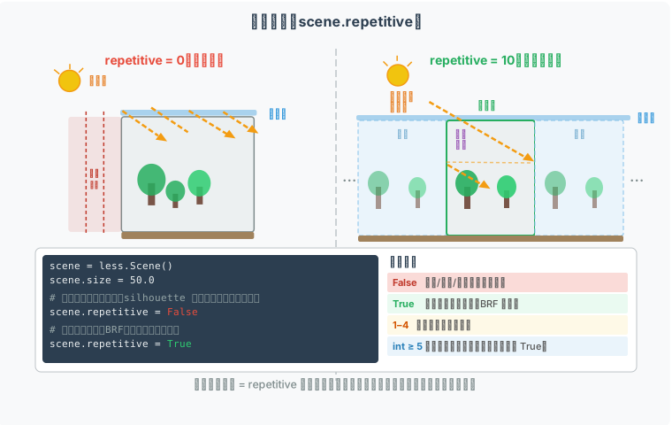
In remote sensing, it is often necessary to simulate homogeneous vegetation canopy (such as large areas of farmland and forests). At this time, the scene should extend infinitely around. LESS achieves this effect through the scene.repetitive parameter: the light will automatically "bend back" when it reaches the scene boundary, which is equivalent to tiling the same scene into an infinite tessellation array.

scene = less.Scene()
scene.size = 50.0          # Scene side length 50m (periodic unit)

# Default: Isolated scene (limited scene, automatically enabled AABB silhouette emission to remove edge darkening)
scene.repetitive = False

# Current public simulation default limited scenario; period modifier released (flat homogeneous terrain only)
# scene.repetitive = True # Infinite tiling (wrap upper limit 100)

How to choose between the two modes?

Finite and periodic scenes have different physical meanings, and the choice depends on what you want to simulate:

Settings	Applicable	Photon Emission Strategy
scene.repetitive = False (default)	Single trees, isolated plots, city blocks, and other real and bounded targets	AABB silhouette: top surface + light-facing side emit evenly, and there is also incident light on the light-facing side of the scene
scene.repetitive = True	Horizontal infinite scene	Published: Rays wrap across boundaries (wrap upper limit 100, you can also set an integer explicitly)

True corresponds to a maximum of 100 ray retracements; integers 1–4 are rejected (native implementation produces black seam artifacts). DEM/grid terrain cannot be repeated or combined with terrain_following.

The old version (≤0.3.1) only scatters photons from the top surface of the scene at repetitive=0. Under oblique sunlight, the part of the light that should have "crossed over the sky and entered the side of the canopy" from outside the scene is lost, and the edge of the scene facing the light will appear systematically dark. In the past, we used repetitive=100 to circumvent this problem - the cost was that the originally limited scene was treated as an infinite cycle, which was physically inaccurate.

Starting from 0.3.2, the limited scene (repetitive=False) will automatically sample photons on the 5 skyward surfaces (top + 4 sides) of AABB:

• Sunlight: Only use 3 sun-facing surfaces (top + sun-facing X side + sun-facing Y side), weighted according to A_face · |d·n|
• Sky light: 5 skyward faces, weighted by area + local hemisphere cos sampling direction of each face

When the ground is flat or the scene is naturally flat (D ≈ 0), the side weight automatically degenerates to 0, which is completely equivalent to the old version; when there is a 3D structure, the side emission makes up for the part of the oblique light that was lost in the past.

After enabling repetitive = True: - Rays that exit the scene boundary will re-enter from the opposite boundary (periodic boundary condition) - Equivalent to the scene being infinitely copied and spliced - The selected backend only stores one copy of the scene geometry and does not occupy additional memory due to periodic copying

Current Public Rules: Default False. Periodic datums for homogeneous canopies use True (wrap 100) or >=5 integers; ALS/LiDAR flight coverage relies on sensor placement rather than scene replication.

Scene elements

Object —— Three-dimensional object

Object is a three-dimensional object in the scene. A Object consists of one or more components (component), each component contains a geometric representation and several attributes:

component = geometry + properties

Components can currently use two geometric representations:

Geometric representation	Description	Common uses
Mesh	Preserve real triangle patches in OBJ	Trunks, branches, explicit leaves, buildings
TurbidBoundary	OBJ only defines a closed space, and statistical parameters (leaf area density, leaf inclination distribution, etc.) are used to describe a large number of small leaves in the space	Large crown, continuous canopy

Both are ordinary components and can be placed in the same Object and use the same set_property(), scene.add() and scene.simulate().

Using Mesh components

When the entire OBJ is used as a Mesh, the abbreviation can be used:

# Load the built-in European ash tree model
tree = less.Object("ash_tree", mesh=less.examples.asset_path("FREX.obj"))

# View component names (automatically scanned from OBJ files)
print(tree.components)  # ['leaves', 'stem_branch']

# Set different properties for different components
tree.set_property("leaves", less.Prospect(cab=40, car=10))
tree.set_property("stem_branch", less.Lambertian(reflectance=0.1))

You can also add specified groups explicitly:

tree = less.Object("ash_tree")
tree.add_component(
    "leaves",
    less.Mesh("tree.obj", group="leaves"),
)
tree.add_component(
    "stem_branch",
    less.Mesh("tree.obj", group="stem_branch"),
)

A OBJ file can contain multiple groups. When group is specified, only the group will be read and will not be added repeatedly. the entire file.

Using the TurbidBoundary component

When the crown contains a large number of leaves and there is no need to preserve the shape of each leaf, you can let OBJ describe only the Closed range:

tree = less.Object("ash_tree")
tree.add_component(
    "crown",
    less.TurbidBoundary("tree.obj", group="crown"),
)
tree.set_property(
    "crown",
    less.OpticalVegetation(
        leaf=less.Prospect(cab=40, car=10),
        leaf_area_density=1.5,              # m²/m³
        leaf_angle_distribution="spherical",
        leaf_size=(0.08, 0.04),             # Length, width, unit m
        leaf_shape="ellipse",
    ),
)

TurbidBoundary is not a separate simulation mode. After creating the scene, still use the normal OpticalImager, BRFSensor, PhotosynthesisProcess or EnergyBalanceProcess. LESS will complete the corresponding calculations based on the geometric representation of the component.

Mixed in one Object

tree = less.Object("tree")
tree.add_component(
    "crown",
    less.TurbidBoundary("tree.obj", group="crown"),
)
tree.add_component(
    "trunk",
    less.Mesh("tree.obj", group="trunk"),
)

tree.set_property(
    "crown",
    less.OpticalVegetation(
        leaf=less.Prospect(cab=40),
        leaf_area_density=1.5,
        leaf_angle_distribution="spherical",
    ),
)
tree.set_property("trunk", less.Lambertian(reflectance=0.12))

The tree crown and trunk will occlude each other in the same simulation and participate in multiple scatterings together. Boundary requirements for statistical vegetation, For blade size, yin and yang blades and accuracy settings see Advanced settings for statistical vegetation .

When adding an object to the scene, you need to specify the position and optionally the scale and rotation:

import numpy as np

# Add multiple trees
positions = np.array([
    [10, 10, 0],
    [20, 15, 0],
    [30, 25, 0],
])
scales = [0.8, 1.0, 1.2]         # Uniform scaling factor for each tree (XYZ equal ratio)
rotations = [0, 90, 180]          # Rotation angle around Z axis (degrees)

handle = scene.add(tree, positions=positions, scales=scales, rotations=rotations)

scales parameters support multiple forms:

Form	Meaning	Example
float	All instances are uniformly scaled	scales=1.5
[N] one-dimensional array, length = number of instances	Uniform scaling of each instance (XYZ equal ratio)	scales=[0.8, 1.0, 1.2] (3 trees)
[N, 3] 2D array	Individual non-uniform scaling of each instance	scales=[[1,1,2],[1,1,1.5],[1,1,3]]

If you need to perform non-uniform scaling on all instances, you can also use a two-dimensional array:

# All trees are stretched twice in the Z direction
scales = [[1.0, 1.0, 2.0]] * len(positions)

scene.add() returns a InstanceHandle, which can be used to modify the instance's transformation after build.

Terrain —— Surface

Terrain represents the ground of the scene. Defaults to flat ground (z = 0), DEM data can also be loaded.

# simple flat ground
terrain = less.Terrain()
terrain.set_property(less.Lambertian(reflectance=0.15))
scene.terrain = terrain

# Or set it directly when creating
scene.terrain = less.Terrain(property=less.Lambertian(reflectance=0.15))

Illumination——Lighting

Illumination defines the lighting conditions of the scene, including direct sunlight and scattered light from the sky.

# Hosek–Wilkie physical sky model (visible light band recommended)
scene.illumination = less.Illumination(
    source=less.Sun(zenith=30, azimuth=150),
    atmosphere=less.HosekWilkieAtmosphere(turbidity=2.5),
)

# Simplified Spectral Atmosphere + Isotropic Scattering (Fast Broadband Simulation)
scene.illumination = less.Illumination(
    source=less.Sun(zenith=30, azimuth=150),
    atmosphere=less.SimpleSpectralAtmosphere(turbidity=2.5),
)

# Vacuum: TOA Direct sunlight does not attenuate and does not produce sky scattering
scene.illumination = less.Illumination(
    source=less.Sun(zenith=30, azimuth=150),
    atmosphere=less.NoAtmosphere(),
)

# Optional 6S atmospheric model
scene.illumination = less.Illumination(
    source=less.Sun(zenith=30, azimuth=150),
    atmosphere=less.SixSAtmosphere(
        atmosphere_profile="midlatitude_summer",
        aerosol_type="continental",
        aot550=0.2,
    ),
)

LESS represents the external radiation environment as “top-of-atmosphere incident sources + atmospheric model”. less.Sun Description only Normal spectral irradiance in the direction of the sun and the top of the atmosphere (TOA); the atmospheric model is responsible for calculating the sun reaching the surface Direct illumination, sky scatter, and model-supported uplink propagation. Both are set uniformly in scene.illumination in:

scene.illumination = less.Illumination(
    source=less.Sun(
        zenith=30,
        azimuth=150,
    ),
    atmosphere=less.Atmosphere.standard(
        "midlatitude_summer",
        aerosol="continental",
        aot550=0.10,
        ground_altitude_km=0.0,
        streams=8,
        sky_mode="anisotropic",
    ),
)

# There is no need to manually prepare surface direct and scattered spectra; simulate() solves by sensor band.
image = scene.simulate(sensor)

It is also possible to solve the atmospheric boundary conditions independently to examine the spectra:

atmosphere = scene.illumination.atmosphere
result = atmosphere.solve(
    [450, 550, 650, 850],
    sun_zenith=30,
)
direct = result.direct_normal_irradiance
diffuse = result.diffuse_horizontal_irradiance

where direct_normal_irradiance is the solar normal direct spectral irradiance, diffuse_horizontal_irradiance is the sky scattering spectral irradiance in the horizontal plane, the units are W m⁻² nm⁻¹. less.Atmosphere can also be used for atmospheric transmittance and path from the surface to the observation height Radiance calculation; complete parameters and output see Atmospheric Model and Earth-Atmosphere Transport .

Model	Applicable scenarios	Description
Atmosphere	Primary layered atmosphere and earth-atmosphere transmission	Shortwave 300–2500 nm; Thermal infrared 3000–14000 nm
SixSAtmosphere	6S parameter system	Requires optional dependency less3d[atmosphere]
HosekWilkieAtmosphere	RGB Visualization, visible light research	320–720 nm directional sky model
SimpleSpectralAtmosphere	Fast broad spectrum lighting	Simplified direct attenuation and isotropic skylight
NoAtmosphere	Vacuum or no-atmosphere experiment	TOA Direct radiation reaches the scene as it is, with zero diffusion
PrescribedAtmosphere	Known atmospheric transmission coefficient	User-given direct and horizontal diffuse transmission coefficient

User specified atmospheric transmission coefficient

When the atmospheric transmission coefficient is known, PrescribedAtmosphere can be used:

scene.illumination = less.Illumination(
    source=less.Sun(
        zenith=30,
        azimuth=150,
        wavelengths=[450, 550, 650, 850],
        irradiance=[1.85, 1.88, 1.55, 1.10],  # TOA normal spectrum, W m⁻² nm⁻¹
    ),
    atmosphere=less.PrescribedAtmosphere(
        wavelengths=[450, 550, 650, 850],
        direct_beam_transmittance=[0.62, 0.70, 0.76, 0.82],
        diffuse_horizontal_transmittance=[0.18, 0.14, 0.10, 0.06],
    ),
)

The reference quantities of the two parameters are different and cannot be mixed:

• direct_beam_transmittance is the direct solar beam transmittance in the usual sense: surface Beam normal direct spectral irradiance divided by TOA beam normal spectral irradiance.
• diffuse_horizontal_transmittance is the horizontal scattering transmission coefficient: surface level The scattered spectral irradiance divided by the projected irradiance of the TOA solar spectrum on the same horizontal plane. it is not "The proportion of scattering in surface illumination".

For a certain wavelength, if the TOA beam normal spectral irradiance is E_toa_normal, and the solar zenith angle is θ, then:

E_direct_normal_surface = E_toa_normal × direct_beam_transmittance
E_diffuse_horizontal_surface = E_toa_normal × cos(θ)
                               × diffuse_horizontal_transmittance

Both are dimensionless coefficients and can be scalars; when using spectral arrays, a reference is also provided. wavelengths, LESS will interpolate to the actual solution wavelength. For those without internal shortwave sources In a passive atmosphere, the sum of the two coefficients for each band cannot be greater than 1. Sun.irradiance always means TOA Beam normal spectral irradiance, total surface irradiance semantics are not accepted.

Property system (Property)

Properties describe the component's behavior during different physical processes.

• geometry describes where the features are and in which spatial representation, such as Mesh or TurbidBoundary。
• property Describe how features reflect light, emit thermal radiation, exchange energy, or perform photosynthesis.

Properties are set on the component. The same component can have properties from multiple physical domains at the same time:

tree.set_property("leaves", optical_property)
tree.set_property("leaves", thermal_property)
tree.set_property("leaves", biophysical_property)
tree.set_property("leaves", physiological_property)

LESS automatically distinguishes them based on the attribute's domain, so there is no need to Repeat the attribute domain name in set_property().

Attribute domain

Attribute domain	Description	Common attributes
optical	reflection, transmission, absorption and scattering of shortwave radiation	Lambertian, Prospect, Fluspect, OpticalVegetation
thermal	Ground object temperature and long wave emissivity	ThermalProperty
microwave	Microwave dielectric, extinction and scattering properties	MicrowaveSoil, MicrowaveVegetation, MicrowaveTrunk
biophysical	Sensible heat, latent heat and surface heat flux exchange parameters	BiophysicalProperty
physiological	Plant physiological parameters such as photosynthesis and stomatal conductance	Farquhar

Features do not need to have all attributes set at the same time. Before the simulation starts, LESS checks the components participating in the process Does it have the required properties?

Band automatic interpolation

All Property in LESS support any band combination, without the need to pre-specify the number of bands when defining properties. During simulation, the properties are automatically interpolated to the wavelength actually used by the sensor, so the same set of properties can be directly used for different sensors such as RGB, multispectral, and hyperspectral.

Optical properties

Optical properties describe the reflection, transmission, absorption and scattering of shortwave radiation by ground objects. Only those involved in optical simulations Only component needs to set optical properties.

# Lambertian: scalar (uniform reflectivity across the entire band)
soil = less.Lambertian(reflectance=0.15)

# Lambertian: Spectral curve (automatic interpolation to analog bands)
import numpy as np
soil_spectral = less.Lambertian(
    reflectance=[0.10, 0.14, 0.18, 0.22, 0.30],
    wavelengths=[400,  550,  670,  800, 1600],   # nm
)

# Lambertian: translucent blade (Lambertian approximation)
leaf_simple = less.Lambertian(
    reflectance=0.08,
    transmittance=0.05,
)

# Prospect: Leaf optical model (spectrum calculated from biochemical parameters, covering 400-2500 nm)
leaf = less.Prospect(
    cab=40,      # Chlorophyll content (μg/cm²)
    car=10,      # Carotenoids (μg/cm²)
    cw=0.012,    # Equivalent water thickness (cm)
    cm=0.008,    # Dry matter content (g/cm²)
    N=1.5,       # Blade structural parameters
)

# RPV: Non-Lambertian BRDF model
brdf_surface = less.RPV(rho0=0.1, k=0.7, theta=-0.15)

# Load from built-in spectral library
lib = less.SpectrumLibrary()
lib.list_spectra()          # View available spectra
green_leaf = lib.as_property("birch_leaf_green")

For Mesh, the optical properties act on the triangular patch:

tree.add_component(
    "leaves",
    less.Mesh("tree.obj", group="leaves"),
)
tree.set_property("leaves", less.Prospect(cab=40))

For TurbidBoundary, the closed boundary defines the extent within which statistical vegetation exists. Leaf optics, leaf area density And the blade inclination angle distribution is described by OpticalVegetation:

tree.add_component(
    "crown",
    less.TurbidBoundary("tree.obj", group="crown"),
)
tree.set_property(
    "crown",
    less.OpticalVegetation(
        leaf=less.Prospect(cab=40),
        leaf_area_density=1.5,              # m² leaf / m³ canopy
        leaf_angle_distribution="spherical",
    ),
)

Complete boundary requirements, blade dimensions and accuracy settings are available in Advanced settings for statistical vegetation .

Thermal properties

Thermal attributes describe the temperature and long-wave emissivity of ground objects, heating infrared, energy balance and other temperature-dependent properties. process use. The temperature unit is K.

# fixed temperature
leaf_thermal = less.ThermalProperty(
    emissivity=0.98,
    temperature=303.15,
)

# Use air temperature during operation
air_coupled_thermal = less.ThermalProperty(
    emissivity=0.98,
    temperature="air",
)

# Explicitly set sun and shade leaf temperatures; both must be provided
split_leaf_thermal = less.ThermalProperty(
    emissivity=0.98,
    temperature_sunlit=308.0,
    temperature_shaded=299.0,
)

# The same component can set both optical and thermal properties
tree.set_property("leaves", leaf)           # Optics
tree.set_property("leaves", leaf_thermal)   # hot

ThermalProperty.temperature is the temperature state of the component and is also energy balanced Initial iteration temperature. The fixed temperature process uses it directly; when set to "air", the runtime starts from Microclimate reads air temperature. After the energy balance converges, the solution result becomes the current patch temperature, which is provided for Used in subsequent photosynthetic or thermal infrared simulations. Temperature and emissivity are only set in ThermalProperty, BiophysicalProperty does not save these two quantities repeatedly.

temperature_sunlit and temperature_shaded are used for thermal infrared with known yin and yang leaf temperatures. Simulation, must be set in pairs, the unit is also K. For Mesh blades, native transmission is evaluated at each hit point Whether it is directly illuminated by the sun, then select the corresponding temperature; for TurbidBoundary, the model uses sun leaves Probabilistic treatment of two conditional temperatures. temperature remains as the base temperature and energy balance of the component Initial value; explicit shade and shade leaf temperatures will not replace this base state.

If the temperature needs to be dynamically determined by environmental conditions and leaf physiological processes, there is no need to guess two temperatures in advance, Instead run energy balance:

microclimate = less.Microclimate(
    air_temperature=25.0,  # °C
    humidity=60.0,         # %
    wind_speed=1.5,
)
energy = scene.simulate(
    less.EnergyBalanceProcess(),
    microclimate=microclimate,
)

sunlit_temperature = energy.result.temperature_sunlit
shaded_temperature = energy.result.temperature_shaded
sunlit_fraction = energy.result.sunlit_fraction

temperature_sunlit and temperature_shaded in the energy balance results are in the sun leaf and The condition temperature obtained under shade leaf radiation conditions; sunlit_fraction describes the temperature of the two in the current space unit. weight. Thermal IR and subsequent coupling processes can use this solution directly.

Microwave properties

Microwave properties describe the dielectric and scattering properties of ground objects in the microwave band. Only microwave simulations need to set this property. The same component can have optical, thermal, and microwave properties simultaneously.

tree.set_property(
    "crown",
    less.MicrowaveVegetation(
        components=[
            less.MicrowaveLeaf(
                radius=0.03,
                thickness=0.0002,
                density=100.0,
                moisture=0.5,
            ),
        ],
        lad="spherical",
    ),
)

Microwave properties describe scattering and dielectric behavior; microwave processes requiring physical temperature to be read simultaneously ThermalProperty. If component is set to ThermalProperty, its current temperature Will be used to microwave vegetation and tree trunks; when not set, uses the temperature in the microwave scatterer. The soil can still be The surface-deep temperature gradient is retained in MicrowaveSoil.

Passive microwave's polarization can be "H", "V", "HV" or "full". "full" returns the four Stokes components of I、Q、U、V, simultaneously passing Tb_H and Tb_V Provides linearly polarized brightness temperature. Active microwave's "full" returns HH、HV、VH、VV, do not confuse the two.

Biophysical properties

BiophysicalProperty describes the way in which ground objects exchange energy with the environment, such as blade width, heat exchange surface, The surface heat flux between the stomata and the surface. It is mainly used for energy balance and dynamic leaf temperature calculations.

tree.set_property(
    "leaves",
    less.BiophysicalProperty(
        two_sided=True,
        stomata_side="bottom",
        leaf_width=0.05,
    ),
)

Different configurations are available for trunks, soil and walls:

tree.set_property(
    "trunk",
    less.BiophysicalProperty(
        two_sided=False,
        stomata_side="none",
    ),
)

Physiological attributes

Physiological properties describe how plants use absorbed photosynthetically active radiation. Farquhar provides C3 plant photosynthesis and Ball–Berry stomatal conductance parameter.

tree.set_property(
    "leaves",
    less.Farquhar(
        Vcmax25=60,
        Jmax25=120,
        Rd25_ratio=0.015,
        BallBerrySlope=9.0,
        BallBerryIntercept=0.01,
    ),
)

Components without physiological properties do not participate in photosynthetic calculations. For example, a tree trunk can have optical properties and thermal property, but Farquhar is usually not set.

What attributes are required for different simulation processes?

The "must" in the following table only applies to the components participating in the corresponding process. For example, when calculating canopy photosynthesis, The canopy must have physiological properties, but buildings that do not participate in photosynthesis do not need to set Farquhar.

Simulation process	optical	thermal	microwave	biophysical	physiological
Optical Imaging, BRF	Required	—	—	—	—
LiDAR Point Cloud and Waveform	Required	—	—	—	—
Shortwave radiation field, APAR	Required	—	—	—	—
Static Photosynthesis	Required	Required	—	Optional	Required
Dynamic Photosynthesis	Must	Must	—	Must	Must
Energy Balance	Required	Required	—	Required	Optional
Thermal Infrared Imaging	—	Required	—	—	—
SIF	Required	By temperature mode	—	By temperature mode	Required
Passive Microwave	—	Required	Required	—	—
Active Microwave	—	Optional	Required	—	—

"Optional" means that the procedure can use additional parameters provided by this attribute, but can still use the simplification without this attribute calculate. "By temperature mode" means that only thermal attributes are required for fixed temperature calculations, and biological properties are also required for dynamic temperature calculations. physical properties.

Complete blade component

The following leaf components can be used for optical imaging, static photosynthesis, and dynamic energy balance:

tree.add_component(
    "leaves",
    less.Mesh("tree.obj", group="leaves"),
)

tree.set_property(
    "leaves",
    less.Prospect(cab=40, car=10, cw=0.012, cm=0.008),
)
tree.set_property(
    "leaves",
    less.ThermalProperty(emissivity=0.98, temperature=303.15),
)
tree.set_property(
    "leaves",
    less.BiophysicalProperty(
        two_sided=True,
        stomata_side="bottom",
        leaf_width=0.05,
    ),
)
tree.set_property(
    "leaves",
    less.Farquhar(Vcmax25=60, Jmax25=120),
)

Properties are set independently by physical domain, so you can modify only the temperature without changing the optical parameters, or you can just modify chlorophyll content without changing energy exchange parameters.

Sensor (Sensor / Imager)

The sensor consists of two parts: projection method and spectral band.

Projection method

# Orthographic projection (default vertical viewing)
ortho = less.Orthographic(image_size=512)

# Perspective projection (camera)
persp = less.Perspective(
    resolution=1024, fov=35,
    position=(25, 60, 20),     # camera position
    target=(25, 25, 5),        # Observe target point
)

# Fisheye projection (hemispheric observation)
fisheye = less.Fisheye(image_size=512, fov=180)

Spectral band

# Custom discrete bands
bands = [475, 560, 668, 842]

# Predefined satellite sensors and their SRF internal sampling interval
sentinel2 = less.OpticalImager(
    less.Orthographic(image_size=512),
    bands=less.Sentinel2A(),
    spectral_resolution=5,
)
landsat8 = less.OpticalImager(
    less.Orthographic(image_size=512),
    bands=less.Landsat8_OLI(),
    spectral_resolution=5,
)

# hyperspectral
bands = less.Hyperspectral(start=400, stop=2500, step=10)

Combined into Imager

# Optical imager = projection + band
sensor = less.OpticalImager(
    less.Orthographic(image_size=512),
    bands=[650, 550, 450],      # RGB
    quality=256,                 # Number of photons (the larger, the more accurate, the slower)
)

# Thermal infrared imager
sensor = less.ThermalImager(
    less.Orthographic(image_size=512),
    bands=[10600],              # 10.6 μm
)

Output product (Product)

All simulate() calls return a Product object:

image = scene.simulate(sensor)

# save as file
image.save("output.png")      # PNG (RGB automatic tone mapping)
image.save("output.tif")      # GeoTIFF (retain original radiation value)

# Get original data (NumPy array)
data = image.data              # shape: (height, width, bands)
print(data.shape, data.dtype)

Different sensors return different types of products:

Sensor	Product Type	Data Content
OpticalImager	ImageProduct	Radiance/reflectance of each band
ThermalImager	ImageProduct	Thermal radiation brightness temperature
BRFSensor	BRFProduct	Multi-angle reflectivity
LiDARSurvey	PointCloud	xyz coordinates + intensity
RadiationFieldSensor	RadiationFieldProduct	Blade-by-blade irradiance

LAI Measurement

LESS can calculate leaf area index (LAI) directly from a 3D scene:

lai = scene.measure(less.LAIMeasurement())
print(f"Scenario LAI = {lai:.2f}")

# Group by component
lai_detail = scene.measure(less.LAIMeasurement(group_by='component'))
print(lai_detail)  # {'leaves': 3.2, 'stem_branch': 0.8}

The same scene can contain both Mesh and TurbidBoundary. Explicit surfels are calculated based on the area of ​​one side of the triangle; Turbid media is calculated as "effective volume within the scene range × leaf_area_density". The boundary shell itself is not part of the leaf area. If the turbid medium crosses the limited scene, only the part that remains in the scene after cropping will be counted; in the periodic scene, the cross-border part will be counted first. Fold back to the base unit. When multiple media overlap in space, the leaf areas represented by each are added together.

property_filter uses the same semantics for both representations. For example property_filter=less.Prospect Matches both explicit PROSPECT blades and OpticalVegetation(leaf=less.Prospect(...)) The ones in represent leaves.

Concept summary

Next step

With these core concepts in hand, let's start the actual simulation:

• 05 - First Simulation: Bare Earth RGB Image
• 02 - Installation and environment configuration
• API refer to

Related API

• less.Scene.simulate(): Automatically build and execute simulations on demand
• less.Scene.build(): Optional advance preparation steps
• less.Scene.rebuild(): Forced refresh of geometry and acceleration structures
• less.Scene.update_instances(): Dynamic instance updates in built scenes
• less.Scene、less.Object、less.Terrain
• less.Mesh、less.TurbidBoundary
• less.Lambertian、less.Prospect、less.RPV
• less.Illumination、less.Sun、less.NoAtmosphere
• less.Atmosphere、less.AtmosphereResult、less.SixSAtmosphere
• less.PrescribedAtmosphere、less.SimpleSpectralAtmosphere、less.HosekWilkieAtmosphere
• less.ThermalProperty、less.Microclimate、less.EnergyBalanceProcess
• less.OpticalImager、less.ThermalImager、less.LAIMeasurement