11b - Upstream and downstream irradiance maps (IrradianceMap)¶

This chapter introduces IrradianceMapSensor - recording the downlink and uplink radiation fluxes at each location in the scene using pixel grid. This function corresponds to the classic version of LESS's "uplink and downlink radiation products" and is commonly used for local solar radiation analysis on complex terrain, understory PAR distribution, and ground-canopy flux modeling.

Physical meaning and recording rules¶

IrradianceMapSensor divides the scene into uniform grids on the XY plane, and each grid is called a pixel. Each pixel maintains two accumulators:

Downward ↓: the incident flux that enters the pixel and interacts;
Upward ↑: The flux emitted from the previous hit pixel and across to the next pixel.

Recording rules (forward photon tracking):

IrradianceMap diagram

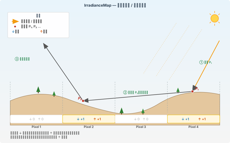
Every time a photon hits \(P\), the current flux is accumulated in the pixel ↓ to which \(P\) belongs.
If the previous hit \(P_{\text{prev}}\) and \(P\) belong to different pixels, then the same flux will be accumulated in the pixel ↑ to which \(P_{\text{prev}}\) belongs.
If \(P\) and \(P_{\text{prev}}\) belong to the same pixel (intra-pixel scattering), they are not recorded (neither ↓ nor ↑ is counted).
When the photon escapes from the scene, if it has hit at least once before, the current flux will be accumulated in the pixel ↑ where the last hit is located.

This rule is the flux convention for LESS2 classical forward photon tracking (photonrt_proc.cpp); IrradianceMapSensor uses the same product definition on the OptiX, Vulkan, and Embree paths of LESS.

How turbid media spans pixels¶

TurbidBoundary can span any number of IrradianceMap cells. The boundary triangle is only responsible for marking the entry of light or Leaving the medium, no radiative interaction is recorded. The real statistical leaf scattering occurs inside the medium, which pixel the scattering point falls on, Which pixel the downward flux belongs to.

When a photon travels from one interaction point to another pixel, the flux leaving the previous pixel column is credited to the previous pixel's upwelling. If the two interactions are still within the same cell, they do not cross the cell column boundary and no additional upward movement is recorded. therefore:

Changing the grid resolution only redistributes the spatial position, and the total downlink energy and the total amount of direct and diffuse energy remain conserved;
The uplink plot describes the flux across the cell column boundaries, the fine grid has more internal boundaries and its spatial sum can be different from the coarse grid;
Limited scenes will first crop out-of-border Turbid volumes, periodic scenes will be split into basic tiles first, and double boundary shells will not be generated across scene boundaries;
When multiple Turbid media overlap, the extinction coefficients are added, and the actual scattering events are only attributed to the selected medium and the pixel where it is located.

Unit and area normalization¶

product.downwelling / upwelling stores the total flux of the pixel column in W/nm (equal to horizontal irradiance × pixel XY area). To get W/m²/nm (area-normalized irradiance), call the _irradiance() method of product to specify which area to divide by:

`surface=`	Divisor	Physical meaning	Data source
`'horizontal'` (default)	`dx · dy` (cell XY area)	irradiance on horizontal plate; standard for "solar radiation diagram"	No additional data required
`'slope'`	`dx · dy / cos(β)`	Pyranometer readings attached to sloping terrain	`terrain.dem` Automatic gradient; or user-supplied `slope` radian map
`'surface'`	∑ DEM triangular surface 3D total area/pixel	Accurate DEM surface area normalization	Automatically accumulated from DEM 2-triangulation network; or user input `surface_area`

p.downwelling_irradiance()                   # Default horizontal, W/m²/nm
p.downwelling_irradiance('slope')            # Slope; automatically derived from terrain.dem
p.downwelling_irradiance('slope', slope=my_slope_rad)   # User passed slope (rad)
p.downwelling_irradiance('surface')          # DEM real 3D area
p.upwelling_irradiance(...)                  # The same 3 surface options

Broadband integration (spectrum + area normalization in one step):

par = p.downwelling_integrated((400, 700), surface='slope')   # W/m² on slope

Product also exposes two auxiliary fields precomputed from the DEM (None on flat ground):

p.terrain_slope — [ny, nx] radians
p.terrain_surface_area — [ny, nx] m² (accurate accumulation of DEM triangular surfaces)

Basic API¶

import numpy as np
import less

scene = less.Scene()            # Automatic selection; also available explicitly using optix/vulkan/embree
scene.size = 40.0
scene.terrain = less.Terrain(property=less.Lambertian(reflectance=0.15))
scene.illumination = less.Illumination(source=less.Sun(zenith=30, azimuth=180), atmosphere=less.NoAtmosphere())
sensor = less.IrradianceMapSensor(
    bands=[550, 850],           # Band (nm)
    grid=(40, 40),              # Method A: Explicitly specify the number of pixels
    # or
    # resolution=0.5, # Method B: meters/pixel (grid derived from scene.size)
    photons_per_m2=400,         # Number of photons projected per m² of scene
    # num_photons=200_000, # Optional: Explicit total photon number, override photons_per_m2 after setting
    max_bounces=None,           # The upper limit of recording depth; None=unlimited (only max_depth/RR limit)
)
product = scene.simulate(sensor)

# output
product.downwelling                         # [ny, nx, nb]  W/nm per pixel
product.upwelling                           # [ny, nx, nb]  W/nm per pixel
product.downwelling_irradiance()            # [ny, nx, nb]  W/m²/nm (horizontal)
product.wavelengths                         # [nb]
product.cell_size                           # (dx, dy) m

Parameters¶

Parameters	Meaning	Typical values
`bands`	Band (nm) list or `SpectralBands` object	`[550, 850]`
`grid`	Number of horizontal pixels `(nx, ny)`	`(100, 100)`
`resolution`	Meter/pixel (choose one from `grid`, `resolution` takes priority)	`0.5`
`photons_per_m2`	Photons per m² scene	`400–4000`
`num_photons`	Optional explicit total photon number; overrides `photons_per_m2`	`200_000`
`max_bounces`	Maximum number of recorded hits (`None` = no limit)	`None` or `1`

grid vs resolution - For resolution: the pixel side length is fixed to the physical scale (e.g. 0.5 m/pixel), grid parameters are ignored; nx = round(scene_width / resolution). - gives grid: explicit pixel number. Pixel side length = scene.size / nx. - Give neither: default grid=(100, 100).

Relationship between max_bounces and depth of LESS2 - max_bounces=1 - records only the first interaction (direct sun/sky radiation reaching the cell), equivalent to depth == 1 for LESS2. - max_bounces=k - First \(k\) interactions to participate in splat; 1 more still tracked to catch escape uplink. - max_bounces=None - Full multiple scattering until end of Russian roulette or max_depth.

Complete example: Flat Lambert surface¶

import math
import numpy as np
import less

# Scene: Flat + Lambertian reflectance 0.15, pure direct light (no sky)
scene = less.Scene()
scene.size = 40.0
scene.terrain = less.Terrain(property=less.Lambertian(reflectance=0.15))

# The spectral parameters are prepared according to the band used in this simulation.
# Sun.irradiance in vacuum is the TOA beam normal irradiance; the horizontal plane flux must also be multiplied by cos (zenith angle)
horizontal = np.array([1.6203, 0.719], dtype=np.float32)
scene.illumination = less.Illumination(
    source=less.Sun(
        zenith=30, azimuth=180, wavelengths=[550, 850],
        irradiance=horizontal / math.cos(math.radians(30))),
    atmosphere=less.NoAtmosphere(),
)

sensor = less.IrradianceMapSensor(
    bands=[550, 850], resolution=1.0,   # 1 m/pixel → 40×40
    photons_per_m2=400, max_bounces=None,
)
p = scene.simulate(sensor)

# Analytical test: Projection of the normal irradiance of the TOA beam results in direct horizontal irradiation; uplink = REFL × this value
E_expected = np.array([1.6203, 0.7190])
print("horizontal down (W/m²/nm):",
      p.downwelling_irradiance().mean(axis=(0, 1)))     # ≈ E_expected
print("horizontal up   (W/m²/nm):",
      p.upwelling_irradiance().mean(axis=(0, 1)))       # ≈ 0.15 × E_expected

Supporting script: scripts/11b_irradiance_map.py

albedo plot on DEM¶

When running IrradianceMapSensor on undulating terrain, a strong slope shadow effect can be observed; and the albedo map can be calculated by pixel-by-pixel up / down to verify the physical consistency (albedo ≡ ρ of each pixel under uniform Lambertian).

import numpy as np
import less
from scipy.ndimage import gaussian_filter

# Synthesize a piece of undulating DEM (you can also pass the GeoTIFF path)
def make_dem(size_m, n=128, seed=42):
    rng = np.random.default_rng(seed)
    dem = np.zeros((n, n), dtype=np.float64)
    for sigma, amp in [(18, 6), (9, 3), (4, 1.5), (2, 0.5)]:
        dem += amp * gaussian_filter(rng.standard_normal((n, n)), sigma=sigma)
    dem -= dem.min()
    dem *= 12.0 / dem.max()
    return dem.astype(np.float32)

scene = less.Scene()
scene.size = 100.0
scene.repetitive = False                     # Limited terrain: Silhouette launch automatically supplements the edge of the oblique launch
scene.terrain = less.Terrain(
    property=less.Lambertian(reflectance=0.30),
    dem=make_dem(100.0),
)
scene.illumination = less.Illumination(source=less.Sun(zenith=45, azimuth=180), atmosphere=less.PrescribedAtmosphere(direct_beam_transmittance=1.0 - (0.0), diffuse_horizontal_transmittance=0.0))
sensor = less.IrradianceMapSensor(
    bands=[550], resolution=0.78,             # ≈ DEM resolution
    photons_per_m2=2000, max_bounces=None)
p = scene.simulate(sensor)

# Three types of area normalization
down_h = p.downwelling_irradiance('horizontal')[:, :, 0]      # W/m² horizontal
down_s = p.downwelling_irradiance('slope')[:, :, 0]           # W/m² slope
down_a = p.downwelling_irradiance('surface')[:, :, 0]         # W/m² DEM 3D

# Albedo = up/down (the ratio is independent of the area convention; cell-by-cell should ≈ rho = 0.30)
up_h   = p.upwelling_irradiance('horizontal')[:, :, 0]
albedo = up_h / np.maximum(down_h, 1e-10)
print("albedo mean:", np.nanmean(albedo))    # ≈ 0.30

Verification script: tests/validation/val16_terrain_albedo.py

observe: - The gap between the maximum value (sunny slope) and the minimum value (shady slope) of downstream down_h often reaches 500× (the shaded area drops to a few thousandths). - down_h (horizontal plane) is the brightest; down_s (slope = down_h × cos β) is slightly darker; down_a (DEM 3D area) is the smallest and most accurate. - Per-pixel albedo is strictly equal to ρ under all three definitions (mathematical conservation of the splat rule: up = ρ × down holds per-pixel).

Backend selection¶

IrradianceMapSensor supports three backends:

scene = less.Scene(backend='optix')   # NVIDIA OptiX
scene = less.Scene(backend='vulkan')  # NVIDIA / AMD / Intel GPU
scene = less.Scene(backend='embree')  # Multithreaded CPU

All three use the same product definition and energy accounting rules, and the results should be consistent within the analytical tolerance or Monte Carlo noise range. OptiX is the production first choice on NVIDIA; Vulkan provides a cross-vendor path to GPU but is still Experimental; Embree does not require GPU. Available before running scene.can_use("irradiance_map") Obtain a single usability conclusion in the current environment.

Difference from `RadiationFieldSensor`¶

Features	`IrradianceMapSensor`	`RadiationFieldSensor`
Output dimensions	2D (nx × ny)	3D (nx × ny × nz)
Original unit	W/nm per pixel column	W/m²/nm per voxel
Record object	Incoming/outgoing flux per hit	Absorbed energy per voxel
Typical applications	Up/downlink radiation, terrain radiation	fPAR, vertical radiation profile

Both are forward photon tracking products and can be selected on demand.

DEM and sensor resolution¶

Relationship between DEM and scene.size: DEM (numpy array or GeoTIFF) is strictly stretched to the XY boundary corresponding to scene.size (vertices are on np.linspace(0, scene_w, n_dem_x)). x_origin / pixel_size read from GeoTIFF will be read but discarded and not used for scene positioning. Therefore, a DEM of (128, 128) is on a 100 m scene, and the DEM vertex spacing is ≈ 100/127 = 0.787 m.

Sensor resolution is decoupled from DEM resolution: You can use any sensor resolution (or grid) to observe the same DEM. When the two are inconsistent, _derive_terrain_geometry internally uses bilinear interpolation to map the slope and triangular area to the sensor grid.

FAQ¶

**Q: Will the accumulation of upward movement exceed that of downward movement? ** Won't. Each scattering is accompanied by albedo attenuation (throughput × ρ). As the number of scatterings increases, the total uplink energy always converges to a value that does not exceed the total downlink energy.

**Q: Why is "intra-pixel scattering" not recorded? ** Avoid double recording of the same pixel "self-in, self-out". For users who treat the pixel as a closed radiation budget unit, this rule makes down − up equal to the net absorption within the pixel.

**Q: Why are max_bounces=1 and infinite scattering almost the same under flat-earth Lambertian? ** The flat Lambertian surface has no geometric structure that can intercept photons again, and the photons basically escape directly after the first scattering. In scenes with canopy or undulations, multiple scattering differences will be apparent.

Q: Under uniform Lambertian, why is the albedo diagram strictly equal to ρ everywhere instead of being higher? ** Because the splat rule pairs records down and up at every scattering event (up = down × ρ holds event-by-event), regardless of scene geometry, up/down = ρ strictly holds after pixel-by-pixel summation. To see a scene where albedo deviates significantly from ρ, you need **non-uniform reflectivity (such as different materials in different slope directions) or examine scene level (∑up / ∑down, which will be lower than ρ due to valley radiation trapping).

Next step¶

12 - Thermal infrared simulation

less.IrradianceMapSensor
less.Scene.simulate()、less.Terrain
less.Illumination、less.Sun、less.PrescribedAtmosphere、less.Lambertian
less.IrradianceMapProduct.downwelling、less.IrradianceMapProduct.upwelling