17 - Reconstruction of 3D scene from LiDAR point cloud¶
less.lidar Converts the LiDAR point cloud (any ALS/TLS/UAV source is acceptable) into a 3D scene for LESS simulation: terrain + canopy envelope + leaf filling. Input .las/.laz file and output less.Scene which can directly run simulate().
Install optional dependencies first
less.lidar uses laspy / scipy / trimesh / cloth-simulation-filter (CSF ground filtering), which is not provided by pip install less3d by default. Install first:
```bash
pip install less3d[lidar]
```
See Chapter 2 § Optional extensions for details.
1. Reconstruction pipeline overview¶
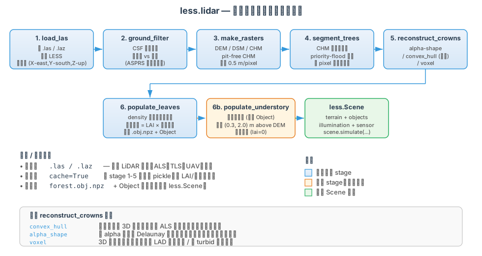
| Stage | Function | What to do |
|---|---|---|
| 1 | load_las |
Read .las/.laz, return to LESS coordinate system |
| 2 | ground_filter |
CSF cloth simulation, ground vs vegetation classification |
| 3 | make_rasters |
DEM / DSM / pit-free CHM |
| 4 | segment_trees |
CHM watershed looking for single wood |
| 5 | reconstruct_crowns |
Canopy geometry (alpha-shape/convex_hull/voxel) |
| 6 | populate_leaves |
Density-weighted sampling leaves within the crown |
| 6b | populate_understory |
Understory shrubs (optional) |
Each stage is a pure function and can be run alone or with a shuttle from_las().
2. Minimal usage¶
Sample data download
Sample point cloud used for demonstration in this chapter: als_plot.las (1.6 MB, about 123×108 m forest stand). After downloading, place it in the working directory and the following code can be run directly.
import less
from less import lidar

scene = lidar.from_las("als_plot.las", lai=2.0)
scene.illumination = less.Illumination(source=less.Sun(zenith=30, azimuth=180), atmosphere=less.NoAtmosphere())
sensor = less.OpticalImager(
    projection=less.Orthographic(resolution=0.5),
    bands=[550, 650, 850], quality=32,
)
img = scene.simulate(sensor).to_brf()
less.save_image(img, "render.png", false_color=[2, 1, 0])
Output (default is in the <las_basename>_lidar/ directory):
plot_lidar/
├── forest.obj.npz ← All leaf geometry (npz binary, scene.build reads directly)
├── understory.obj.npz ← If enabled understory_lai>0
└── .cache/ ← stage 1-5 result pickle (when cache=True)
Take a look at the scene in the browser¶
Before running simulate(), first use scene.show() to open the interactive viewer to see the reconstruction effect (whether the terrain, canopy envelope, and leaf distribution are reasonable):
Three tabs:
- Scene —— 3D geometry browsing, you can hide/show terrain and each Object, drag and rotate with the mouse
- Render——Simple preview, quickly test light angle and spectrum
- Simulate —— Equipped with sensor to run formal simulation, and the results will be displayed on the spot
For detailed usage, see 15 - Interactive Visualization .
3. Important parameters¶
3.1 LAI / Blade¶
lidar.from_las("plot.las",
    lai=2.0,              # Scene-level LAI (including forest windows, most commonly used)
    # lad=1.5, # or: volume density m²/m³ (consistent for each tree)
    # lai_per_tree={1: 2.0, 2: 3.5, ...}, # Or: by tree_id alone
    leaf_area=0.05,       # Single leaf area m² (default 0.01 = 100 cm²)
    leaf_shape="square",  # "square" (2 triangles) / "disk" (12 triangles)
    leaf_angle="spherical",   # Angle distribution
    jitter_sigma=None,    # density sampled Gaussian jitter radius (m)
)
Large scenes with high LAI will generate millions of blades.
leaf_shape="square"+ Increaseleaf_area(0.05-0.1) is a commonly used speed-increasing combination.
3.2 Reconstruction method and leaf sampling¶
There are two parameters that work together and should be understood together:
method—— How to reconstruct canopy geometry (calculate volume, draw contours)sampling——Where to put the blades**
lidar.from_las("plot.las", lai=2.0,
    method="convex_hull",     # "convex_hull" / "alpha_shape" / "voxel"
    sampling="density",       # "density" / "uniform"
)
Three types method¶
method |
Description | Applicable |
|---|---|---|
convex_hull |
Whole tree convex hull | Default; sparse ALS (≤ 5 pts/m²), no points lost |
alpha_shape |
Delaunay tetrahedrons filtered by alpha threshold |
Dense point cloud (≥ 20 pts/m²) / TLS, capable of capturing canopy depressions |
voxel |
3D occupation grid | Want to control LAD directly by pressing voxel |
Two kinds of sampling¶
sampling |
Where to put the blades |
|---|---|
density (default) |
Randomly picked from the LiDAR return point of this tree + Gaussian jitter jitter_sigma |
uniform |
Uniform sampling within the volume (tetrahedron/voxel) generated by method |
Combination effects¶
method + sampling |
What determines the blade position | The role of method |
|---|---|---|
convex_hull + density (default combination) |
LiDAR point distribution | Only affects volume → Total blade number fine-tuning |
alpha_shape + density |
LiDAR point distribution | Only affects volume → Fine-tuning of total blade number |
voxel + density |
LiDAR point distribution | Only affects volume → Fine-tuning of total blade number |
convex_hull + uniform |
Delaunay uniform within the tetrahedron | Determine the filling range (convex hull) |
alpha_shape + uniform |
Uniform within the retained tetrahedron | Determine the filling range (including depressions) |
voxel + uniform |
Uniform within each voxel AABB | Determine the filling range (discrete grid) |
Want to see the visual effects of method?
Under the default sampling="density", the three methods are almost visually identical - the blades are all near the LiDAR return point. To see the method difference, cut sampling="uniform".
LAI conservation: No matter which combination, the total leaf area = LAI × scene area is strictly unchanged. The sampling method only determines where the leaves are.
3.3 Understory (optional)¶
lidar.from_las("plot.las", lai=2.0,
    understory_lai=0.3,                   # 0 off (default)
    understory_height_range=(0.3, 2.0),   # Height above ground m
    understory_leaf_area=0.02,
    understory_leaf_angle="planophile",
)
The understory is independently populate_understory - 1 Object, and the leaf density follows the actual low LiDAR return distribution.
3.4 Flatland vs DEM¶
normalize=True: Subtract the DEM value of its XY position from each point z (the point cloud is normalized to the flat ground), and the final scene uses flat terrain. Suitable for plot-scale simulation (does not care about terrain fluctuations, rendering faster).
normalize=False (default): Keep the real DEM and enter the terrain mesh into the scene.
3.5 Cache (strongly recommended to enable)¶
Pickle the stage 1-5 product (points / rasters / segmentation / crowns) to <basename>_lidar/.cache/pipeline_<hash>.pkl. The Cache key does not contain leaf parameters, so adjusting LAI / leaf spectrum / leaf_angle can hit the cache and reappear the scene in a few seconds.
The cache will only be invalidated when you change the geometry parameters (resolution / method / min_tree_height / normalize, etc.).
3.6 Default parameter list (simplest call)¶
Equivalent to:
| Parameters | Default | Description |
|---|---|---|
resolution |
0.5 | DEM/CHM m/pixel |
method |
"convex_hull" | Canopy geometry |
min_tree_height |
2.0 | CHM threshold m |
min_tree_distance |
3.0 | Minimum horizontal distance between tree tops m |
leaf_area |
0.01 | Single leaf area m² |
leaf_shape |
"square" | 2 triangle/leaf |
leaf_angle |
"spherical" | |
understory_lai |
0.0 | Close understory |
normalize |
False | Reserve DEM |
cache |
False | Do not cache |
write_obj |
False | Only write npz, do not write OBJ text |
output_mode |
"merge" | Merge all leaves into one Object |
4. Staged API (for experts, easy to cache intermediate results)¶
pc      = lidar.load_las("plot.las")
pc      = lidar.ground_filter(pc)               # Default is CSF
rasters = lidar.make_rasters(pc, resolution=0.5)
seg     = lidar.segment_trees(rasters,
                              min_height=2.0,
                              min_distance=3.0)
crowns  = lidar.reconstruct_crowns(
              pc, seg,
              method="convex_hull",
              rasters=rasters,                  # Must be passed, otherwise sub-canopy will not filter
              min_canopy_height=2.0,
              understory_layer=False)

crowns.save("plot.crowns")        # pickle caches reconstruction results

# --- This is the only step for subsequent adjustment of LAI ---
crowns = lidar.Crowns.load("plot.crowns")
forest_obj, forest_pos = lidar.populate_leaves(
    crowns,
    lai=2.0, leaf_area=0.05,
    out_path="forest.obj")

# Make your own Scene
import numpy as np
scene = less.Scene()
scene.size = pc.extent
scene.terrain = less.Terrain(
    property=less.SpectrumDB("dark_soil_mollisol"),
    dem=rasters.dem.astype(np.float32))
scene.illumination = less.Illumination(source=less.Sun(zenith=30, azimuth=180), atmosphere=less.NoAtmosphere())
scene.add(forest_obj, positions=forest_pos)
The staged API and
from_lasproducts are completely equivalent - except that the former allows you to pickle the intermediate results (such ascrowns) separately and rerunpopulate_leaveswhen adjusting the spectrum/blade parameters.
5. Modify the spectrum after reconstruction¶
The constructed scene can change the leaves/surface spectrum without rebuilding:
forest = scene.objects["forest"]

# Switch tree species spectrum
forest.set_property("leaves", less.SpectrumDB("larch_leaf_green"))
# or physical blade model
forest.set_property("leaves", less.Prospect(cab=15))   # Yellowing
# Change the surface
scene.terrain.set_property(less.SpectrumDB("loam_brown"))

img = scene.simulate(sensor)   # Automatically reuse paths without rebuilding BVH
For details, see 16 - Scene and Project: Parameter hot updates and geometry reconstruction.
6. Performance Tips¶
| Scene | Parameter adjustment suggestions |
|---|---|
| Iterative experiment of adjusting LAI | cache=True, blade parameters can be changed at will |
| High LAI (≥ 3) large scenes | leaf_area=0.05, leaf_shape="square" |
| Want to visualize geometry | write_obj=True (use Blender to open the generated OBJ) |
| Don’t want to write disk | Directly use staged API, and finally populate_leaves(write_obj=False) only produces npz |
| The crowned leaves are unpleasant | constrain_to_hull=True (note that LAI may be lost when the jitter is large) |
7. Currently known limitations¶
| Limitations | Description |
|---|---|
| Only canopy reconstruction | No trunk/branch geometry (LiDAR reflection itself is difficult to distinguish these) |
| Single component | By default all blades are in one g leaves group. output_mode="groups" can be grouped by species/tree |
| LAI source | Must be specified manually by the user (choose one of three lai / lad / lai_per_tree); inversion from LiDAR is not supported |
| understory does not distinguish individual trees | There is one Object in the understory of the entire forest, which cannot be controlled independently by bushes |
8. A complete demo¶
import os, less
from less import lidar

scene = lidar.from_las(
    "als_plot.las",      # See §2 for sample data download
    lai=1.5, understory_lai=0.5,
    normalize=True, cache=True,
)
scene.illumination = less.Illumination(source=less.Sun(zenith=45, azimuth=180), atmosphere=less.NoAtmosphere())
sensor = less.OpticalImager(
    projection=less.Orthographic(resolution=0.5),
    bands=[550, 650, 850], quality=32,
)

# 1) Default rendering
img1 = scene.simulate(sensor).to_brf()
less.save_image(img1, "out/01_baseline.png", false_color=[2, 1, 0])

# 2) Change the spectrum and try again (without rebuilding BVH, in seconds)
scene.objects["forest"].set_property("leaves", less.SpectrumDB("larch_leaf_green"))
scene.terrain.set_property(less.SpectrumDB("loam_brown"))
img2 = scene.simulate(sensor).to_brf()
less.save_image(img2, "out/02_larch_loam.png", false_color=[2, 1, 0])

# 3) Save as a Project that can be edited (including named sensor)
project = less.Project(
    scene=scene,
    title="Plot 01 baseline",
    author="qijb",
)
project.add_sensor(sensor, name="Nadir multispectral")
project.save_directory("out/plot01.less")
Relevant chapters: 16 - Scene and Project (parameter hot update, engineering resources and Project Format v2).
Related API¶
less.lidar.reconstruct()、less.lidar.preprocess()less.lidar.estimate_lai()、less.lidar.build_scene()less.Scene、less.Projectless.SpectrumDB、less.Prospect、less.Terrainless.save_image()