05 - First Simulation: Bare Earth RGB Image

This chapter will complete your first radiative transfer simulation with minimal coding. We will create a simple bare earth scene, generating a RGB image.

Simulation principle

In the simplest case, the scene consists of a flat surface. Sunlight illuminates the ground, and the radiance reflected from the ground is received by the orthophoto sensor to form an image.

Orthographic projection imaging

Orthographic sensors view the scene from directly above. All the observation rays are parallel to each other - just like a satellite observing the ground from an extremely high altitude.

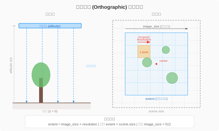
The meaning of key parameters:

• image_size: Number of pixels of the image (for example, 256 means 256×256 pixels)
• extent: Ground imaging range (meters), the default is equal to scene.size
• resolution: Ground resolution (meter/pixel), choose one from image_size
• center: Imaging center point, the default is the center of the scene

extent = image_size × resolution. If the scene is 50m, image_size=500, then resolution = 0.1 m/pixel.

RGB band

To generate the RGB image, we need to specify the center wavelengths of the red, green, and blue bands. In LESS, the bands are arranged in the order given by the list:

bands = [650, 550, 450]  # Band 1 = Red (650nm), Band 2 = Green (550nm), Band 3 = Blue (450nm)

Complete code

import less

# 1. Create a scene
scene = less.Scene()
scene.size = 10.0                         # 10m × 10m scene

# 2. Set ground properties
# Lambertian: uniform reflection in all directions
# reflectance=0.3 means reflecting 30% of the incident light
scene.terrain = less.Terrain(
    property=less.Lambertian(reflectance=0.3)
)

# 3. Set up lighting
# sun_zenith=30: Sun altitude angle 60°
# sun_azimuth=150: The sun is in the southeast direction
scene.illumination = less.Illumination(source=less.Sun(zenith=30, azimuth=150), atmosphere=less.SimpleSpectralAtmosphere(turbidity=2.0))

# 4. Configure the sensor and simulate (the first call will automatically build the scene)
sensor = less.OpticalImager(
    less.Orthographic(image_size=256),     # 256×256 pixels
    bands=[650, 550, 450],                 # R, G, B
    quality=64,                            # Number of photons (the tutorial uses low values ​​to speed things up)
)
image = scene.simulate(sensor)

# 5. Save results
image.save("bare_soil_rgb.png")
print("Simulation completed!")

Supporting script: scripts/05_first_simulation.py

Code interpretation

Scene and Terrain

less.Scene() creates an empty scene. scene.size = 10.0 sets the scene ground range to 10m × 10m.

less.Terrain() creates a surface. Lambertian(reflectance=0.3) is the simplest optical property - Lambertian, that is, the reflectivity is the same in all directions. reflectance=0.3 means reflecting 30% of the incident light.

SimpleSpectralAtmosphere lighting model

Illumination(Sun, SimpleSpectralAtmosphere) contains two components:

1. Direct Sunlight: The direction is determined by sun_zenith (zenith angle) and sun_azimuth (azimuth angle)
2. Diffuse Sky Light: Automatically calculated based on a simplified spectral atmosphere model (Rayleigh + aerosol + ozone + water vapor), approximately uniform in all directions

Use NoAtmosphere() under vacuum conditions; use when the transmission coefficient of TOA to the surface is known PrescribedAtmosphere. Sun.irradiance is always TOA beam normal spectral irradiance.

simulate()

scene.simulate(sensor) will automatically prepare the scene and build the acceleration structure on the first call, then perform Monte Carlo ray tracing and return the results. Ordinary simulation does not require calling scene.build() in advance; use scene.rebuild() when forced refresh of externally modified geometry files is required. For details, see Scene Life Cycle .

quality parameter

quality controls the number of photons emitted by each pixel. Larger values ​​result in lower image noise but longer computation time.

quality	noise level	applicable scenarios
16-64	Obvious noise	Quick preview, tutorial demonstration
128-256	Lower noise	General analysis
512-2048	Negligible noise	Publication quality

Output product

Save as image

image.save("output.png")     # PNG (automatically tone mapped to 8-bit)
image.save("output.tif")     # GeoTIFF (retain original physical quantities)

Access raw data

import numpy as np

data = image.data
print(f"Data shape: {data.shape}") # (256, 256, 3)
print(f"Data type: {data.dtype}") # float32
print(f"Data range: {data.min():.4f} ~ {data.max():.4f}")

The radiance value (W/m²/sr/nm) is returned instead of the pixel value from 0-255. This is a primitive physical quantity that can be used for quantitative analysis.

Try to modify parameters

Thanks to the digital twin architecture, you can directly modify parameters and re-simulate without rebuilding:

# Change the position of the sun
scene.illumination = less.Illumination(source=less.Sun(zenith=60, azimuth=90), atmosphere=less.SimpleSpectralAtmosphere(turbidity=2.0))
image2 = scene.simulate(sensor)
image2.save("bare_soil_low_sun.png")

# Change ground reflectivity
scene.terrain.set_property(less.Lambertian(reflectance=0.1))
image3 = scene.simulate(sensor)
image3.save("bare_soil_dark.png")

Add a plant

Let's add a corn plant to bare ground and see the effect:

# Load the built-in corn model
maize = less.Object("maize", mesh=less.examples.asset_path("maize.obj"))
maize.set_property(less.Prospect(cab=40, car=8, cw=0.012, cm=0.006, N=1.5))

# Place a tree in the center of the scene
scene.add(maize, positions=[[5.0, 5.0, 0.0]])
scene.rebuild()  # Geometry changes require rebuild

image4 = scene.simulate(sensor)
image4.save("one_maize.png")

In the next chapter we will cover the configuration of terrain and optical properties in more detail.

Next step

• 06 - Terrain and optical properties

Related API

• less.Scene、less.Terrain、less.Object
• less.Lambertian、less.Prospect
• less.Illumination、less.Sun、less.SimpleSpectralAtmosphere
• less.Orthographic、less.OpticalImager
• less.Product.save()、less.Product.to_brf()