32 - Energy balance and leaf temperature
Thermal simulations need the temperatures of the surfaces in the scene. Temperatures can be prescribed (chapter 26) or solved from an energy balance driven by illumination, air temperature, humidity and wind speed. This chapter covers the second way.
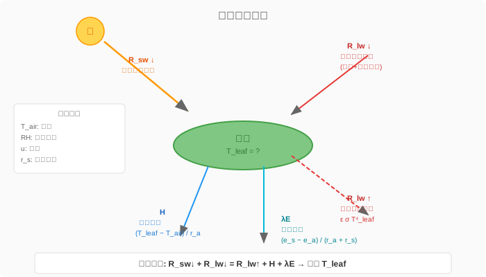
What is solved
For every leaf or ground element taking part, LESS finds the temperature that balances the energy budget:
- R_n: net radiation, absorbed shortwave and longwave minus emitted longwave;
- H: sensible heat flux, set by the temperature difference between surface and air and the exchange resistance;
- LE: latent heat flux, i.e. transpiration or evaporation, set by stomatal resistance and the vapour pressure deficit;
- G: soil heat flux, zero for leaves.
Longwave exchange between leaves, ground and sky is computed in the 3-D scene, so the temperature of one leaf affects the leaves and ground around it.
Required properties
Components taking part in the energy balance need three kinds of property: optical, thermal and biophysical:
import less

scene = less.Scene()
scene.size = 6.0
scene.terrain = less.Terrain(property=less.Lambertian(reflectance=0.15))
scene.terrain.set_property(less.ThermalProperty(temperature="air", emissivity=0.95))
scene.terrain.set_property(less.BiophysicalProperty(two_sided=False, stomata_side="none",
                                                    ground_heat_fraction=0.35))
scene.illumination = less.Illumination(
    source=less.Sun(zenith=30, azimuth=150),
    atmosphere=less.SimpleSpectralAtmosphere(turbidity=2.0))

plant = less.Object("plant")
plant.add_component("leaves", less.Mesh(less.asset_path("tutorial_tree.obj"), group="leaves"))
plant.set_property("leaves", less.Prospect(N=1.5, cab=45, car=10, cw=0.012, cm=0.006))
plant.set_property("leaves", less.ThermalProperty(temperature="air", emissivity=0.98))
plant.set_property("leaves", less.BiophysicalProperty(
    leaf_width=0.05, stomata_side="bottom", stomatal_resistance=150.0))
scene.add(plant, positions=[(3, 3, 0)])
ThermalProperty.temperature is the starting temperature of the solution: "air" starts from the air temperature; a temperature in kelvin can also be given.
BiophysicalProperty describes how a surface exchanges energy with its surroundings:
| Parameter | Meaning |
|---|---|
two_sided |
Both faces take part in radiative exchange (true for leaves; the ground is always one-sided) |
stomata_side |
Face with stomata: "top", "bottom", "both" or "none" (no transpiration) |
stomatal_resistance |
Stomatal resistance or soil surface resistance (s m⁻¹) |
leaf_width |
Characteristic leaf width (m), used for the boundary-layer resistance r_a = 200 √(d/u) |
aerodynamic_resistance |
Exchange resistance given directly (s m⁻¹), replacing the leaf-width formula |
ground_heat_fraction |
G as a fraction of net radiation |
ground_heat_flux |
Constant G (W m⁻²), as an alternative to the previous parameter |
solve |
When false, the temperature stays at the value in the thermal property and is not solved |
Common settings:
| Object | two_sided |
stomata_side |
G |
|---|---|---|---|
| Leaves | Yes | bottom |
0 |
| Soil | No | none or top |
Fraction or constant |
| Stems | Yes | none |
0 |
| Water | No | top |
0 |
Microclimate
climate = less.Microclimate(
    air_temperature=25.0,   # °C
    humidity=60.0,          # relative humidity, %
    wind_speed=2.0,         # m s⁻¹
    pressure=101325.0,      # Pa
    ca=400.0,               # CO₂, ppm
)
downwelling_longwave (W m⁻²) gives the downward longwave radiation from the sky; when it is not given, it is estimated from air temperature and humidity.
Solving
energy = scene.simulate(less.EnergyBalanceProcess(quality="preview"), microclimate=climate)
result = energy.result
print(result.summary())
quality can be "preview", "standard" or "high"; n_samples_per_face (longwave samples per face of each triangle), max_iterations, convergence_tol (K) and energy_tolerance (W m⁻²) can also be set directly.
After solving, thermal imaging uses the solved temperatures automatically:
thermal = scene.simulate(less.ThermalImager(
    less.Orthographic(image_size=64), bands=[10600.0], quality=32), microclimate=climate)
thermal.to_brightness_temperature(unit="K").save("leaf_temperature.png")
Results
import numpy as np

area = np.asarray(result.primitive_areas)
temperature = np.asarray(result.temperatures) - 273.15
print("temperature range (°C):", temperature.min(), temperature.max())

for name in ("R_n", "H", "LE", "G"):
    print(name, "total (W):", float(np.sum(np.asarray(getattr(result, name)) * area)))
| Result | Meaning |
|---|---|
temperatures |
Temperature of each element (K) |
R_n, H, LE, G |
Fluxes per unit area (W m⁻²) |
S_abs, L_abs, L_emit |
Absorbed shortwave, absorbed longwave, emitted longwave |
primitive_areas |
Area of each element (m²) |
temperature_sunlit, temperature_shaded, sunlit_fraction |
Temperatures of the sunlit and shaded parts and the sunlit fraction |
residual, converged, n_iterations |
Energy budget residual, whether it converged, number of iterations |
Check that the energy budget closes:
active = result.active_mask
print("largest residual (W m⁻²):", abs(result.residual[active]).max())
print("converged:", result.converged, "iterations:", result.n_iterations)
If the solution does not converge, less.ConvergenceError is raised; check the microclimate and starting temperatures, or increase max_iterations.
Statistical vegetation
Statistical vegetation is used in the same way, and results are given per component: the temperatures of sunlit and shaded leaves are solved separately within the component and then combined by sunlit fraction.
canopy = less.Object("canopy")
canopy.add_component("crown", less.TurbidBoundary(less.asset_path("tutorial_tree.obj"), group="crown"))
canopy.set_property("crown", less.OpticalVegetation(
    leaf=less.Prospect(cab=45), leaf_area_density=1.5, leaf_angle_distribution="spherical"))
canopy.set_property("crown", less.ThermalProperty(temperature="air", emissivity=0.98))
canopy.set_property("crown", less.BiophysicalProperty(leaf_width=0.05, stomata_side="bottom",
                                                      stomatal_resistance=150.0))
scene.add(canopy, positions=[(3, 3, 0)])

mixed = scene.simulate(less.EnergyBalanceProcess(quality="preview"), microclimate=climate)
print(mixed.result.summary())
One scene can contain triangle-mesh leaves, statistical vegetation and terrain together, and they exchange radiation in a single solution.
Canopy surface layer and atmospheric stability
The leaves above use the leaf width to compute boundary-layer resistance. To study the exchange between a whole canopy and the atmosphere, use the canopy surface layer model of SCOPE: the canopy exchanges sensible and latent heat with the air at the reference height through a canopy resistance, the soil through a soil resistance, and the Monin–Obukhov length computed from the sensible heat flux of the whole scene corrects the resistances for atmospheric stability.
field = less.Scene()
field.size = (1.0, 1.0)
field.repetitive = True
field.terrain = less.Terrain(property=less.Lambertian(reflectance=0.15))
field.terrain.set_property(less.ThermalProperty(temperature="air", emissivity=0.94))
field.terrain.set_property(less.BiophysicalProperty(two_sided=False, stomata_side="top",
                                                    stomatal_resistance=500.0,
                                                    ground_heat_fraction=0.35))
field.illumination = less.Illumination(
    source=less.Sun(zenith=30, azimuth=180, irradiance=0.4), atmosphere=less.NoAtmosphere())

from pathlib import Path
Path("canopy_box.obj").write_text(
    "g canopy\n"
    + "".join(f"v {x} {y} {z}\n" for x, y, z in [(0, 0, 0), (-1, 0, 0), (-1, 2, 0), (0, 2, 0),
                                                  (0, 0, -1), (-1, 0, -1), (-1, 2, -1), (0, 2, -1)])
    + "f 1 4 3\nf 1 3 2\nf 5 6 7\nf 5 7 8\nf 1 5 8\nf 1 8 4\n"
    + "f 2 3 7\nf 2 7 6\nf 1 2 6\nf 1 6 5\nf 4 8 7\nf 4 7 3\n")
crop = less.Object("crop")
crop.add_component("leaves", less.TurbidBoundary("canopy_box.obj", group="canopy"))
crop.set_property("leaves", less.OpticalVegetation(
    leaf=less.Prospect(cab=45), leaf_area_density=1.5, leaf_angle_distribution="spherical"))
crop.set_property("leaves", less.ThermalProperty(temperature="air", emissivity=0.98))
crop.set_property("leaves", less.BiophysicalProperty(leaf_width=0.1, stomata_side="bottom",
                                                     stomatal_resistance=600.0))
field.add(crop, positions=[(0.0, 0.0, 0.0)])

layer = less.SurfaceLayer(canopy_height=2.0, leaf_area_index=3.0, measurement_height=5.0)
calm = less.Microclimate(air_temperature=25.0, humidity=50.0, wind_speed=0.5,
                         downwelling_longwave=350.0, surface_layer=layer)
coupled = field.simulate(less.EnergyBalanceProcess(quality="preview", max_iterations=100),
                         microclimate=calm)
print(coupled.metadata["surface_layer"])
Main parameters of SurfaceLayer:
| Parameter | Meaning |
|---|---|
canopy_height, leaf_area_index |
Canopy height (m) and leaf area index |
measurement_height |
Height at which wind speed and air temperature are measured (m), above the canopy |
roughness_length, displacement |
Roughness length and zero-plane displacement (m); computed from the canopy parameters as in SCOPE when not given |
drag_coefficient, soil_boundary_resistance, within_canopy_resistance |
Leaf drag coefficient, soil boundary-layer resistance, within-canopy resistance |
stability |
Whether atmospheric stability is taken into account, true by default |
With a surface layer, do not also give aerodynamic_resistance for leaves and soil. coupled.metadata["surface_layer"] gives the final Obukhov length, friction velocity, canopy resistance, soil resistance and the sensible heat flux of the scene. In daytime, when the canopy is warmer than the air, the atmosphere is unstable, resistances fall and leaves become cooler; at low wind speeds this can amount to 1–2 °C. Because the Obukhov length is iterated together with the temperatures, set max_iterations to 60–100.
When to solve again
After changing the illumination, microclimate, properties, geometry or instances, the previous result no longer applies and must be solved again. LESS raises an error if an outdated result is passed to a sensor.