Appendix A7 - Fluorescence generation and transport

After absorbing sunlight, a leaf emits fluorescence from both faces. Reflection, transmission and reabsorption between leaves then modify the fluorescence observed by a sensor. This case starts with one leaf plane, adds a second and third layer, and introduces a black slit to compare spatial images against an exact geometric reference.

Scene and inputs

Drag to rotate, or open the scene separately. Horizontal periodic boundaries represent infinite uniform leaf layers. The slit scene uses a finite leaf and open boundaries.

Condition	Setting
Leaves and ground	Horizontal 4 m × 4 m leaves above black absorbing ground
Layers and heights	One, two or three layers, at 3, 2 and 1 m
Leaf parameters	FLUSPECT, N = 1.5, car = 10, cw = 0.012, cm = 0.009
Upper, middle, lower layer	cab = 40, 20, 60; static yields = 0.012, 0.018, 0.006
Excitation	450, 550 and 650 nm, each 1 nm wide; normal spectral irradiance 1 W m⁻² nm⁻¹
Sun	Zenith 30°, azimuth 90°; no atmosphere or diffuse sky
Fluorescence observation	687, 740 and 760 nm; 32 × 8 pixels over 3 m × 1 m on the horizontal reference plane
Layer viewing directions	Zenith 0°, 45° and 60°, azimuth 90°
Slit	Width 1.2 m, 0.5 m above the leaf; black absorbing panels
Slit viewing directions	Zenith 0°, 30° and 60°, azimuth 90°
Sampling	4096, 16384 and 65536 excitation rays per triangle face; 256, 1024 and 4096 image samples per pixel

Twelve configurations include doubled-yield, zero-yield and leaf-underside controls. The underside observation uses a perspective sensor at (2, 2, 0.5) m, looking at (2, 2, 3) m with a 30° field of view; other observations are orthographic. Fluorescence paths allow up to 64 surface interactions. Image values are fluorescence radiance in W m⁻² sr⁻¹ nm⁻¹, excluding reflected sunlight.

Reference solutions

Leaf coefficients and fluorescence sources

Leaf reflectance, transmittance and forward/backward excitation–emission coefficients are supplied by FLUSPECT and listed in the leaf coefficient table. Given these inputs, layer excitation and fluorescence transport are calculated independently. See Vilfan et al.'s FLUSPECT-B paper for the leaf model.

For excitation irradiances \(E_i^\downarrow\) and \(E_i^\uparrow\) incident on the upper and lower faces of layer i, absorbed energy is

\[ A_i^{top}=(1-r_i-t_i)E_i^\downarrow,\qquad A_i^{bottom}=(1-r_i-t_i)E_i^\uparrow. \]

With static yield \(\phi_i\), the two fluorescence radiance sources are

\[ S_i^\uparrow=\phi_i\sum_b(M_{b,i}A_{i,b}^{top}+M_{f,i}A_{i,b}^{bottom}), \]

\[ S_i^\downarrow=\phi_i\sum_b(M_{f,i}A_{i,b}^{top}+M_{b,i}A_{i,b}^{bottom}). \]

The coefficient table includes excitation-to-emission photon-energy conversion, normalization by leaf absorptance, and the Lambertian exitance-to-radiance factor \(1/\pi\). This static setup uses total absorbed energy; chlorophyll absorption and within-leaf reabsorption are represented by the FLUSPECT coefficients.

Infinite multiple transport between leaf layers

At each fluorescence wavelength, outgoing upward and downward radiances satisfy

\[ U_i=S_i^\uparrow+r_iD_{i-1}+t_iU_{i+1},\qquad D_i=S_i^\downarrow+t_iD_{i-1}+r_iU_{i+1}. \]

There is no incoming fluorescence at the upper boundary and no reflection from the black lower boundary. Solving the linear system sums all orders of reflection, transmission and reabsorption. The excitation bands use the same layer relations, with normal solar irradiance times the incidence cosine at the upper boundary. Radiance above uniform diffuse layers is independent of viewing direction, providing an angular check as well.

Three-dimensional slit and shadow

Sunlight reaches the leaf through the black slit. With horizontal coordinates relative to the slit centre, slit width w, height h above the leaf, and both sun and observer to the east, illuminated and visible intervals are

\[ I_s=[-w/2-h\tan\theta_s,\ w/2-h\tan\theta_s],\qquad I_v=[-w/2-h\tan\theta_v,\ w/2-h\tan\theta_v]. \]

Their intersection is both illuminated and visible. The leaf is planar and all other surfaces absorb, so there is no indirect excitation or fluorescence reflection between objects. Exact overlap with each pixel gives the reference image, including mixed pixels at the boundaries.

Fluorescence images use randomized Sobol points within pixels. Excitation absorption and subsequent transport use independent random samples.

Results

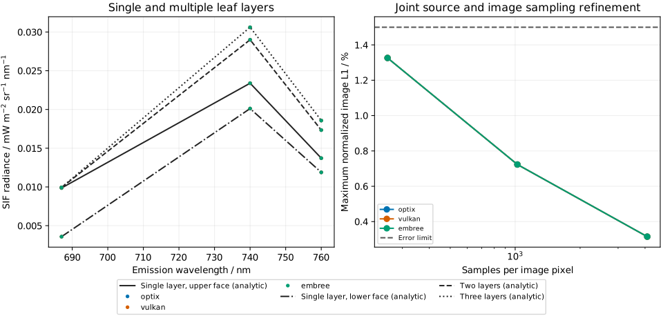
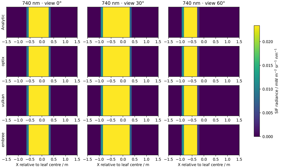
Backend	Excitation error	Mean SIF error	Image L1 error	Final budget change	Result
optix	0.0115%	0.0622%	0.3150%	0.0451%	Pass
vulkan	0.0115%	0.0622%	0.3150%	0.0449%	Pass
embree	0.0115%	0.0622%	0.3150%	0.0451%	Pass

All 36 results pass. All three backends return zero for zero yield and zero relative linearity error when the yield is doubled.

Absorbed-excitation error is normalized by the strongest absorbing leaf face in each band, with a 1% limit; this also evaluates analytically dark faces. Limits are 1% for each band's image-mean radiance and 1.5% for normalized image L1 error. L1 error is the sum of absolute differences across pixels and bands divided by the summed reference radiance. Each band's image mean must change by no more than 0.5% between the final two sampling levels. The zero-yield control uses an absolute limit of 10⁻¹⁰ W m⁻² sr⁻¹ nm⁻¹; doubled-yield relative linearity error must not exceed 10⁻⁵. Input and result files below provide individual checks.

Reproduce

• Inputs and sampling plan
• Fixed leaf coefficients
• Leaf mesh and slit panels
• Reproduction script
• Result data

Keep the relative script and data paths, then run:

python scripts/appendix_fluorescence.py --output results/fluorescence

Use --plot-only results/fluorescence/results.json to regenerate figures with matplotlib.