Appendix A2 - Attenuation and single scattering

As light crosses an absorbing layer, part reaches the ground and the rest is absorbed. This case compares a uniform absorbing medium, a spherical turbid canopy of black leaves, and randomly placed discrete horizontal black leaves. The same layer is then tested with scattering, comparing its first-order radiance across viewing directions.

Photon emission and within-pixel positions use randomized Sobol points; medium collisions and subsequent scattering use independent random samples.

Scene settings

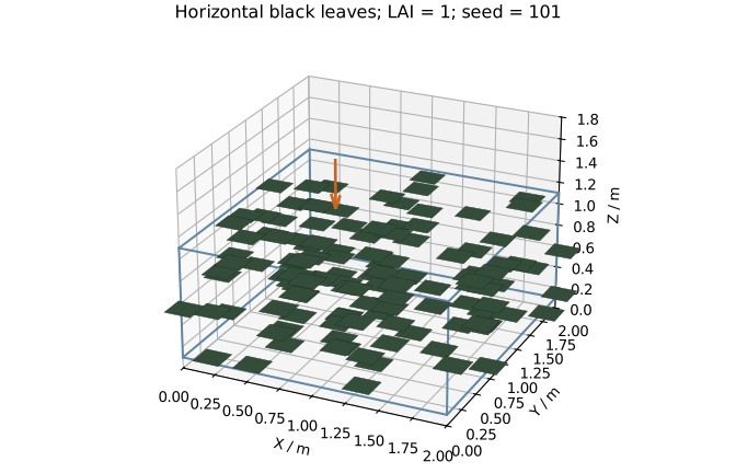
Drag to rotate one of the discrete scenes, or open it separately. The wireframe marks the layer boundary, shared by the uniform medium and turbid canopy.

Condition	Setting
Horizontal cell	2 m by 2 m, periodic X/Y, at most 10000 crossings
Layer	Z = 0.1-1.1 m; thickness H = 1 m
Ground	Perfectly absorbing black surface at Z = 0
Illumination	Collimated 550 nm sunlight; normal irradiance 1 W m^-2 nm^-1; no atmosphere or sky
Solar direction	Zenith 0, 45 and 75 degrees; azimuth 90 degrees
Uniform medium	Absorption coefficient k = 0, 0.1, 1 and 5 m^-1; zero scattering; thermal emission disabled
Turbid canopy	Spherical leaf normals; zero leaf reflectance and transmittance; LAI = 0, 0.2, 2 and 10
Discrete leaves	100 horizontal black squares, side 0.2 m, LAI = 1; independently uniform positions within the layer
Scene ensemble	12 sets of leaf positions, seeds 101-112, shared across backends
Photon budgets	Medium and turbid: 1, 2 and 4 million; each discrete scene: 1 and 4 million; final budget 4 million

Leaves crossing a cell edge include their neighbouring periodic copies, preserving their full area. The physical leaf area per periodic cell remains 4 m2.

Horizontal irradiance is \(E_0\cos\theta\), giving incident flux \(P_0=4E_0\cos\theta\). All fractions below are normalized by the corresponding incident flux.

Analytic solution

Uniform medium and spherical turbid canopy

The path through a layer of thickness H is \(H/\cos\theta\). By Beer-Lambert's law, transmission through a uniform absorber is

\[ T=\exp\left(-\frac{kH}{\cos\theta}\right). \]

For statistical black leaves,

\[ T=\exp\left(-\frac{G(\theta)\,\mathrm{LAI}}{\cos\theta}\right). \]

Spherical leaf normals give \(G=0.5\). Setting \(kH=0.5\,\mathrm{LAI}=\tau\) gives the same transmission in both representations. The four settings correspond to vertical optical depths \(\tau=0,0.1,1,5\), spanning vacuum to strong absorption.

Layer absorptance is \(A=1-T\); the black ground absorbs a fraction T. We also divide the layer into four equal sublayers. For a sublayer with optical depths \(\tau_1,\tau_2\) at its upper and lower boundaries, measured downward from the top,

\[ A_{\mathrm{layer}}=e^{-\tau_1/\cos\theta}-e^{-\tau_2/\cos\theta}. \]

Discrete horizontal leaves

For a horizontal leaf of area a, a ray intersects it with probability \(a/S\), where S is the horizontal cell area. With N independently placed leaves, the ensemble mean transmission is

\[ \mathbb E[T]=\left(1-\frac aS\right)^N. \]

This coverage-probability result follows from the placement used here. With \(a=0.04\,\mathrm{m^2}\), \(S=4\,\mathrm{m^2}\) and \(N=100\),

\[ \mathbb E[T]=0.99^{100}=0.36603234. \]

The mean is independent of solar zenith angle. A particular scene has different overlaps along different paths, so we compare the mean of 12 random scenes with theory.

As individual leaves become smaller and more numerous at fixed \(\mathrm{LAI}=Na/S\), this expression approaches \(e^{-\mathrm{LAI}}\), the statistical limit for strictly horizontal leaves. For LAI = 1, that limit is 0.36787944. The finite-leaf reference in this case is \(0.99^{100}\). Turbid simulations use spherical normals, while horizontal leaves are represented by explicit triangles.

Simulation results

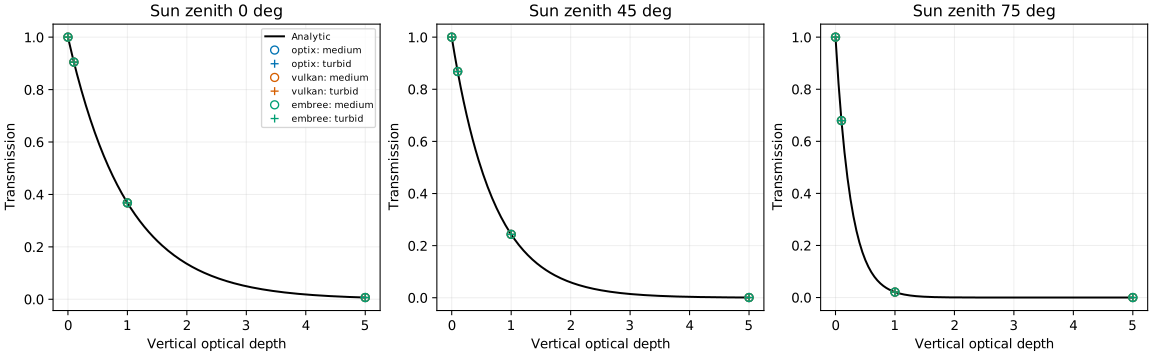
Curves show the analytic transmission; circles and plus signs represent the uniform medium and turbid canopy. Increasing solar zenith lengthens the path and reduces transmission. Backend points overlap closely.

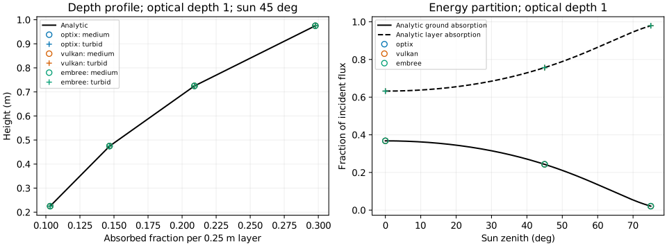
The left panel compares absorption in four sublayers. The right panel shows total layer absorption and flux reaching the black ground.

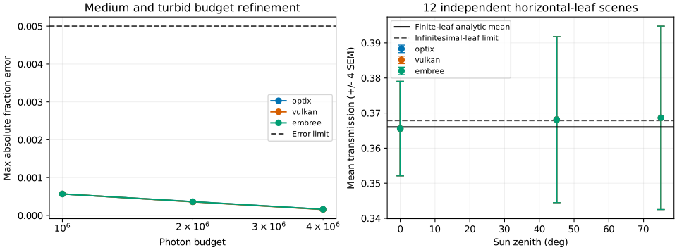
The left panel increases photon count to check medium and turbid errors. The right panel shows mean transmission for discrete leaves, with error bars of four standard errors across scenes. The solid line is the finite-leaf analytic mean; the dashed line is the infinitesimal horizontal-leaf limit.

Error evaluation

Metric	Limit
Maximum absolute error in transmission, total absorption or sublayer absorption	0.005
Uniform-medium versus spherical-turbid transmission or absorption difference	0.005
Maximum change between final photon budgets	0.003
Energy closure error	0.0001
Escaping or truncated flux fraction	0.00001 each
Discrete ensemble mean transmission error	0.005, and within four standard errors across scenes

Transmission is ground absorption divided by incident flux. Layer absorption comes from the recorded grid absorption. The discrete ensemble standard error is \(s/\sqrt{12}\), where s is the sample standard deviation of scene transmissions. Photon-budget refinement and variation among leaf arrangements are evaluated separately.

Backend	Max medium error	Max turbid error	Max representation difference	Max discrete mean error	Status
optix	0.00015934	0.00015354	0.00016901	0.00260122	Pass
vulkan	0.00015508	0.00015230	0.00017426	0.00260119	Pass
embree	0.00015911	0.00015330	0.00016901	0.00260109	Pass

Mean transmission for discrete horizontal leaves is shown below; the analytic mean is 0.36603234.

Sun zenith	OptiX	Vulkan	Embree	Largest standard error across scenes
0°	0.36557375	0.36557375	0.36557346	0.00336840
45°	0.36812525	0.36812525	0.36812511	0.00591345
75°	0.36863356	0.36863353	0.36863343	0.00653107

Errors are absolute; final results use 4 million photons per simulation. All three backends meet the evaluation thresholds.

Angular response of a scattering medium

Keep the same 1 m layer and black ground, and divide extinction into absorption and scattering. Let \(\tau=(k_a+k_s)H\) be extinction optical depth and \(\omega=k_s/(k_a+k_s)\) the single-scattering albedo. The comparison uses radiance that leaves the layer after exactly one scattering event, extracted from the simulated first-order component.

Condition	Setting
Illumination, boundaries and wavelength	Same as the layer above; solar zenith 0° and 60°
Main angular sweep	\(\tau=1\), \(\omega=0.7\), phase parameter \(g=-0.5,0,0.5\)
Views	−60°, −30°, 0°, 30°, 60° in the solar principal plane; plus zenith 60° at relative azimuth 90°
Optical-depth controls	\(\tau=0.1,3\), \(\omega=0.7\), \(g=0\)
Scattering-fraction controls	\(\omega=0.2,1\), \(\tau=1\), \(g=0\)
Control directions	Solar zenith 60°; views −60°, 0°, 60°
Sampling	8 × 8 pixels over a 0.1 m width; 128, 512 and 2048 samples per pixel, adopting 2048

Signed viewing angles distinguish the two sides of the principal plane: positive angles share the solar azimuth; negative angles differ by 180°. All views look at the layer from above. Each backend compares 48 input combinations.

Exact first-order solution

Use the Henyey–Greenstein phase function:

\[ p_g(\cos\Theta)=\frac{1-g^2}{4\pi(1+g^2-2g\cos\Theta)^{3/2}}. \]

Here \(\Theta\) is the angle between the incident photon's propagation direction and the outgoing direction. Zero \(g\) is isotropic; positive values favour forward scattering, and negative values favour backward scattering. For solar and viewing zenith angles \(\theta_0,\theta_v\) and relative azimuth \(\Delta\phi\),

\[ \cos\Theta=-\cos\theta_0\cos\theta_v -\sin\theta_0\sin\theta_v\cos\Delta\phi. \]

Let \(\mu_0=\cos\theta_0\), \(\mu=\cos\theta_v\), and let \(t\) be extinction optical depth measured downward from the layer top. Attenuation before and after scattering is \(e^{-t/\mu_0}\) and \(e^{-t/\mu}\), respectively. Thus,

\[ L_1=\frac{E_0\omega p_g}{\mu}\int_0^\tau e^{-t(1/\mu_0+1/\mu)}\,dt =\frac{E_0\omega p_g\mu_0}{\mu_0+\mu} \left[1-e^{-\tau(1/\mu_0+1/\mu)}\right]. \]

Normalizing by irradiance on the horizontal plane gives the first-order BRF:

\[ \mathrm{BRF}_1=\frac{\pi L_1}{E_0\mu_0} =\frac{\pi\omega p_g}{\mu_0+\mu} \left[1-e^{-\tau(1/\mu_0+1/\mu)}\right]. \]

This solution constrains phase-function direction, attenuation along both paths, and the linear dependence on single-scattering albedo.

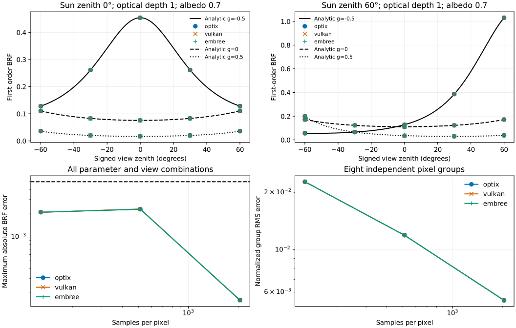
The upper panels compare angular responses at the two solar zenith angles. Black curves are analytic; coloured markers are simulated. The lower panels show maximum BRF error and grouped error as sampling increases. Each image is divided into eight disjoint pixel groups. Their means provide the standard error. Student-t intervals with a Bonferroni correction cover all 144 comparisons at a 1% family-wise error rate.

Metric	Threshold
Maximum absolute first-order BRF error	≤ 0.005
Maximum relative first-order radiance error	≤ 2%
Maximum BRF change between the last two sampling levels	≤ 0.003
Statistical agreement with the analytic value	Inside the simultaneous confidence interval above
Sampling convergence	Final normalized group RMS error and average between-group variance both below the coarsest level

Backend	Maximum absolute BRF error	Maximum relative radiance error	Maximum BRF budget change	Result
optix	0.00015899	0.1893%	0.00240502	Pass
vulkan	0.00015779	0.1893%	0.00241821	Pass
embree	0.00015897	0.1893%	0.00240501	Pass

All 144 comparisons meet these criteria. Each final input combination uses 131072 samples; normalized group RMS error decreases from about 2.28% at the coarsest budget to 0.54%.

Downloads and reproduction

• Inputs and sampling plan
• Layer boundary (OBJ) and horizontal leaf (OBJ)
• Reproduction script
• Result data

Save the script under scripts/, and the inputs and both OBJ files under the sibling data/attenuation/. With LESS, NumPy, SciPy and matplotlib installed, run:

python scripts/appendix_attenuation.py --output build/attenuation

OptiX, Vulkan and Embree must all be available. The script writes one result file and five SVG figures. With the result data downloaded, add --scattering-only to recompute just the scattering section.