Appendix A1 - Analytic validation of a V valley

This example compares LESS simulations with analytic solutions for a simple V valley. One slope reflects according to Lambert's law, while the other is black and absorbs all incoming light. Under vertical sunlight, we can calculate the directional BRF, whole-valley albedo and absorptance.

The following sections describe the scene, derive the reference values and compare results from the OptiX, Vulkan and Embree backends in LESS 3.1.0.

Three-dimensional scene

Explore the valley geometry by dragging or using the arrow keys. You can also open the 3D view separately or download it for offline viewing.

Condition	Setting
Horizontal cell	X and Y each span 0-2 m; valley axis parallel to Y
Slopes	Both 45 degrees; internal opening angle 90 degrees
Elevation	Floor Z = 0.1 m; both rims Z = 1.1 m
Western slope (X < 1 m)	Opaque Lambertian; reflectances 0.2, 0.6 and 0.9 at 550, 850 and 1600 nm
Eastern slope (X > 1 m)	Perfect absorber; reflectance and transmittance both zero
Underlying terrain	Black flat ground at Z = 0, entirely covered by the slopes
Boundary	Periodic X/Y, at most 10000 crossings; an infinitely long valley repeated across X
Illumination	Vertical collimated sunlight; normal irradiance 1 W m^-2 nm^-1 at each wavelength; no atmosphere or sky
Observation	Across-valley signed zenith -70 to +70 degrees in 10-degree steps; positive toward east (azimuth 90), negative toward west (270)
Sampling	1, 2 and 4 million photons for each BRF and flux product; final budget 4 million

The valley consists of four triangles placed above flat terrain. Its horizontal opening is 4 m2, giving an incident flux of 4 W nm^-1 at each wavelength. The three wavelengths are evaluated separately below.

Analytic solution

Radiation within the valley

Sunlight illuminates both slopes uniformly. The black slope absorbs all incident radiation, while the grey slope reflects a fraction according to Lambert's law. Reflected light then escapes through the opening or reaches the black slope and is absorbed. The grey slope therefore has uniform outgoing radiance, which gives the analytic solution below.

Directional BRF

Let slope angle \(\beta=45^\circ\), grey reflectance \(\rho\), and normal solar irradiance \(E_0\). Irradiance on the grey slope is \(E_0\cos\beta\), so its outgoing radiance is

\[ L_g=\frac{\rho E_0\cos\beta}{\pi}. \]

With signed viewing zenith \(\theta\) as defined above, the grey slope occupies the following fraction of the projected opening:

\[ f_g(\theta)=\operatorname{clip}\!\left( \frac{1+\tan\beta\tan\theta}{2},0,1\right). \]

The opening-averaged radiance is \(\bar L=f_gL_g\), hence

\[ \mathrm{BRF}(\theta)=\frac{\pi\bar L}{E_0} =\rho\cos\beta\,f_g(\theta). \]

Below -45 degrees the grey slope is fully hidden and BRF is zero. Above +45 degrees it occupies the entire visible opening and BRF is \(\rho/\sqrt2\). At nadir BRF is \(\rho/(2\sqrt2)\). A valley made of local Lambertian surfaces can therefore have a direction-dependent BRF.

Flux and absorption

For equal-width slopes extending infinitely along the valley axis, Hottel's crossed-string method gives the grey-to-black view factor

\[ F_{gb}=\frac{2l-w}{2l}=1-\cos\beta, \]

where slope length \(l=\sqrt2\) m and opening width \(w=2\) m. For the geometric derivation, see the crossed-string method in NASA's Thermal Radiation Heat Transfer, section 2.

Half of the incoming flux reaches the grey slope, a fraction \(\rho\) is reflected, and a fraction \(1-F_{gb}=\cos\beta\) of that reflection escapes. Whole-valley albedo \(R\) and absorptance \(A\) are therefore

\[ R=\frac{\rho}{2}(1-F_{gb})=\frac{\rho}{2\sqrt2}, \qquad A=1-R. \]

The grey and black slopes absorb fractions \((1-\rho)/2\) and \(1/2+\rho F_{gb}/2\), respectively. Their sum gives whole-valley absorptance.

Wavelength / nm	Grey reflectance	Analytic valley albedo	Analytic valley absorptance
550	0.2	0.07071068	0.92928932
850	0.6	0.21213203	0.78786797
1600	0.9	0.31819805	0.68180195

These reference values are calculated directly from the equations above.

Simulation results

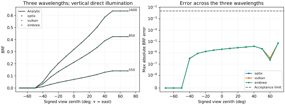
Lines show the analytic reference; colored points show LESS results. The right panel shows the largest error across wavelengths for each angle.

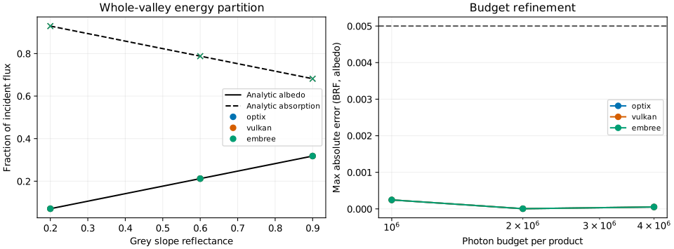
The left panel compares escaping and absorbed flux fractions with theory. The right panel shows maximum BRF/albedo error at the three budgets.

Error evaluation

The following absolute-error thresholds are used to evaluate agreement with the analytic solution.

Metric	Limit
Maximum BRF error across 15 directions and 3 wavelengths	0.005
Maximum albedo / absorptance error across wavelengths	0.005 each
Energy closure \(\lvert R+A+T-1\rvert\)	0.0001
Truncated path flux fraction \(T\)	0.00001
Maximum BRF, albedo or absorptance change between the final two budgets	0.003

Flux is recorded with ForwardRadiationFieldSensor. Escaping flux divided by incident flux gives albedo; the sum of grid and terrain absorption divided by incident flux gives absorptance. \(T\) is the fraction of flux still carried by photons when they reach the path-depth or periodic-crossing limit.

Final results: 4 million photons per product

Backend	Max BRF error	Max albedo error	Max absorptance error	Closure error	Final budget change	Status
OptiX	0.00000728	0.00005252	0.00005249	2.69e-08	0.00005782	Pass
Vulkan	0.00000728	0.00005296	0.00005296	1.42e-08	0.00005782	Pass
Embree	0.00000728	0.00005252	0.00005249	2.69e-08	0.00005782	Pass

All three backends meet the thresholds, with zero truncated flux. Initial photon positions use randomized Sobol points; subsequent scattering uses independent random samples. At 1, 2 and 4 million photons, maximum BRF errors are 0.00000436, 0.00000549 and 0.00000728. The final two budgets differ by at most 0.00005782, below the limit of 0.003.

Downloads and reproduction

• Scene inputs
• Scene model (OBJ)
• Reproduction script
• Result data

Save the script under scripts/, and input.json and scene.obj under the sibling data/v-valley/. With LESS and matplotlib installed, run:

python scripts/appendix_v_valley.py --output build/v-valley

All three backends must be available to run this script. It performs the simulations in sequence and writes result data (JSON) and three comparison figures (SVG), including values, errors and execution details for each photon budget.