A9 - Microwave brightness and polarization

Starting with smooth bare soil, then adding a uniform absorbing vegetation layer, finite blocks and a gap, this case tests surface emission, vegetation absorption/emission, reflected sky radiation and H/V polarization. Bare soil and absorbing layers have independent analytic references; finite blocks also have analytic images including mixed pixels.

Scene and inputs

Drag to rotate, or open the scene separately. Changing incidence angle shows the H/V directions relative to the incidence plane. The scene uses the built-in flat terrain and needs no mesh file.

Setting	Value
Surface	20 m × 20 m horizontal periodic tile, no vegetation
Frequency	1.4 GHz, L band
Soil texture	Sand 30%, clay 20%
Surface model	Smooth specular, RMS height 0 cm
Dielectric model	Hallikainen; independent reference uses published 1.4 GHz coefficients
Temperature	Equal surface/deep temperatures, baseline 290 K
Observation	Orthographic, altitude 30 m, 4 m × 4 m footprint, 4 × 4 pixels
Outputs	H/V brightness, full Stokes and source partition
Background brightness	2.725 K
Pixel sampling	1, 8 and 64 samples per pixel

Fourteen conditions are used:

Group	Moisture / m³ m⁻³	Incidence	Soil / K	Air / K	Nadir atmospheric optical depth
Dry-soil angles, 4 conditions	0.05	0°, 30°, 60°, 75°	290	290	0
Wet-soil angles, 4 conditions	0.30	0°, 30°, 60°, 75°	290	290	0
Cooler/warmer soil, 2 conditions	0.30	60°	280, 320	290	0
Cooler atmosphere	0.30	60°	290	260	0.05
Warmer atmosphere	0.30	60°	290	310	0.20
Azimuth rotation, 2 conditions	0.30	60°	290	290	0

Azimuth defaults to 0°; the final two conditions use 90° and 225°. The atmosphere is an isothermal absorbing layer with prescribed optical depth. Equal surface and deep soil temperatures make effective temperature equal to the specified soil temperature.

Independent analytic reference

Permittivity and Fresnel reflection

The Hallikainen polynomial calculates real permittivity and loss separately from sand/clay percentages and volumetric moisture. Published coefficients and equations are given in JPL's soil-moisture chapter, equations 5.1-17–19 and copied into the inputs. The reference calls neither the LESS dielectric solver nor its Fresnel solver.

For complex permittivity ε, incidence θ and u = √(ε − sin²θ), power reflectivities are

\[ R_H=\left|\frac{\cos\theta-u}{\cos\theta+u}\right|^2,\qquad R_V=\left|\frac{\varepsilon\cos\theta-u}{\varepsilon\cos\theta+u}\right|^2. \]

For an opaque soil half-space, Kirchhoff's law gives eₚ = 1 − Rₚ. H and V coincide at normal incidence and separate at oblique angles; high incidence further tests polarization response.

Surface, sky and atmosphere

Using the microwave Rayleigh–Jeans brightness convention, atmospheric transmission and downwelling sky brightness are

\[ t=\exp(-\tau/\cos\theta),\qquad T_{sky}=T_a(1-t)+T_{bg}t. \]

Sensor brightness for polarization p is

\[ T_{B,p}=t\left[(1-R_p)T_s+R_pT_{sky}\right]+T_a(1-t). \]

The three terms are transmitted surface emission, reflected sky brightness and upwelling atmospheric emission. See the SMAP passive soil-moisture algorithm document for the brightness convention and source contributions.

Polarization and isothermal closure

Full Stokes output satisfies I = T_H + T_V and Q = T_H − T_V, with U = V = 0 here. Stokes V denotes circular polarization, distinct from V-polarized brightness T_V. Requesting H, V, HV or full Stokes separately must retain the corresponding brightness. Rotating viewing azimuth must also preserve H/V brightness for this horizontal isotropic soil.

The isothermal check uses source responses: recover eₚ and Rₚ from the soil and sky contributions and check eₚ + Rₚ = 1. Recombining both responses at a common temperature T must return T. This is an isothermal recombination check using linear transport; actual simulations retain the specified sky background.

Results

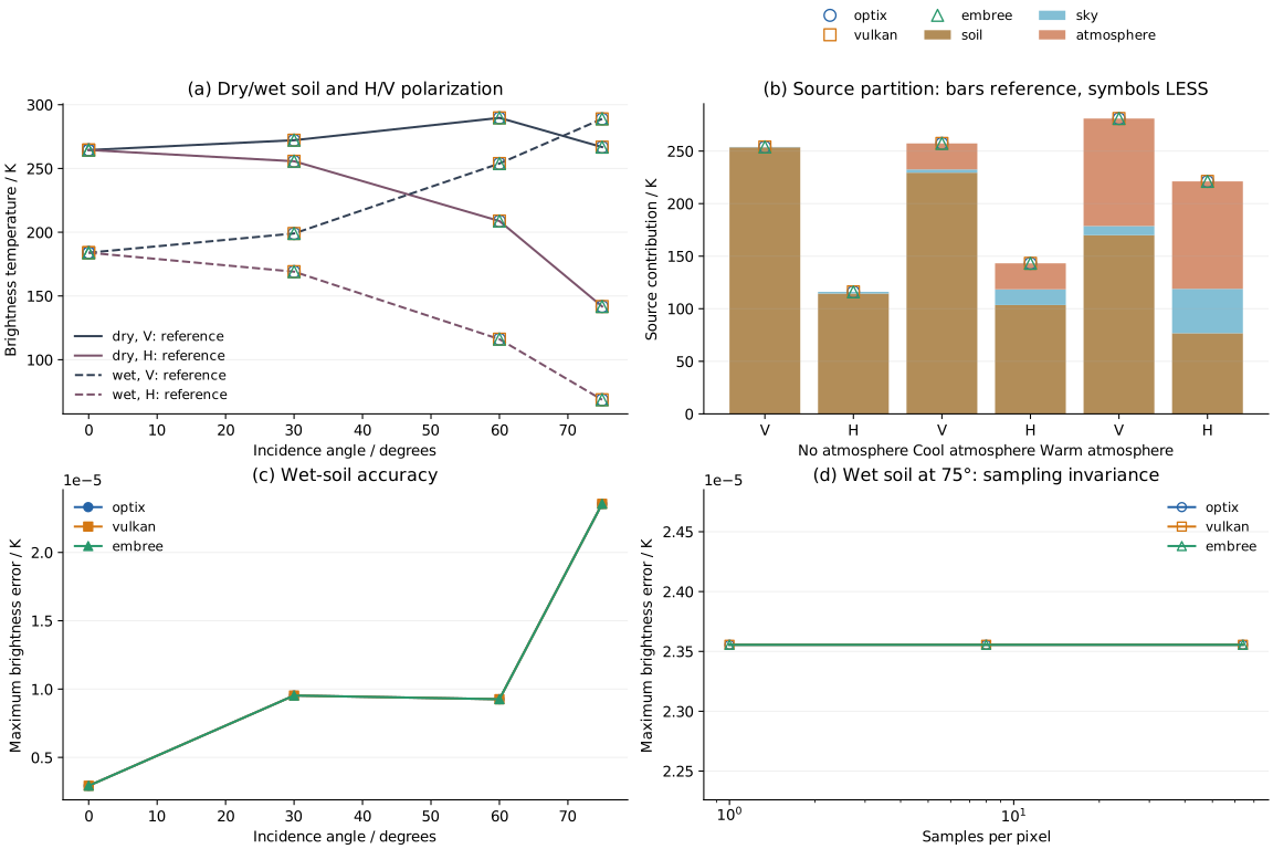
Backend	H/V brightness error / K	Source error / K	Reflectivity error	e + R closure error	Result
optix	0.00002356	0.00001348	3.354e-08	5.075e-08	Pass
vulkan	0.00002356	0.00001348	3.354e-08	5.075e-08	Pass
embree	0.00002356	0.00001348	3.354e-08	5.075e-08	Pass

All 42 adopted comparisons pass. Errors are maxima over fourteen conditions, all pixels and polarization channels for each backend. H/V brightness and source limits are 0.001 K; reflectivity must agree within 10⁻⁵ and |e + R − 1| within 10⁻⁶. Full-Stokes error is limited to 0.002 K and cross-Stokes error to 10⁻⁵ K.

Sampling stability

Increasing samples per pixel from 1 to 8 and 64 gives zero final brightness change. Wet soil at 75° and the warmer-atmosphere condition are also repeated with three independent seeds, and angular-integration budgets of 16, 64 and 256 at fixed pixel quality. Brightness remains unchanged.

Every ray in this uniform smooth scene sees the same incidence and temperature, with no scattering-integration noise. The remaining error of about 10⁻⁵ K does not change with budget. This checks sampling stability; scattering canopies require a separate convergence study.

Absorbing vegetation and three-dimensional gaps

Select “Uniform layer”, “Single block” or “Two blocks and gap” in the preview above. These simulations explicitly use volume_scattering=False, retaining particle absorption, thermal emission and soil reflection. Absorption coefficients are calculated independently from vegetation permittivity and the Rayleigh spheroid model.

Scene and conditions

Leaves have radius 2 mm, thickness 0.2 mm, gravimetric moisture 0.55 and vertical normals. Vegetation occupies z = 1–3 m, with baseline density 800000 m⁻³ and temperature 300 K; wet soil is 280 K. There is no atmosphere and sky brightness is 2.725 K. Viewing azimuth is 90°, with the image referenced to ground level z = 0.

Condition	Incidence	Setting
Uniform layer, 3 conditions	0°, 40°, 60°	Full 20 m × 20 m periodic tile
Denser layer	40°	Density 2000000 m⁻³
Cooler leaves	40°	Vegetation 280 K, soil 310 K
Equal vegetation/soil temperature	40°	Both 290 K; sky remains 2.725 K
Single finite block, 3 conditions	0°, 40°, 60°	x = 6.25–9.25 m, y = 0–20 m, open boundaries
Two blocks and a gap, 2 conditions	40°, 60°	Second block x = 11.25–14.25 m; gap 2 m

Finite-block images cover x = 4–16 m and y = 9–11 m with 24 columns × 4 rows. Each pixel is 0.5 m × 0.5 m; block edges pass through pixels, testing exact half-covered areas.

Independent references

The reference uses the Ulaby–El-Rayes dual-dispersion dielectric model and electrostatic spheroid dipoles. With leaf volume V, χ = ε − 1 and transverse/axial depolarization factors \(L_t\) and \(L_z\), polarizabilities are \(\alpha_t=V\chi/(1+L_t\chi)\) and \(\alpha_z=V\chi/(1+L_z\chi)\). For horizontal leaves, using ε = ε′ − iε″,

\[ \kappa_H=-nk\operatorname{Im}(\alpha_t),\qquad \kappa_V=-nk\operatorname{Im}(\alpha_t\cos^2\theta+\alpha_z\sin^2\theta), \]

where n is number density and k is wavenumber. The reference calculates these coefficients from inputs without reading LESS particle tables.

Uniform-layer transmission is γₚ = exp[−κₚh/cosθ]. Exact absorption-only brightness is

\[ T_{B,p}=\gamma_p(1-R_p)T_s+ (1-\gamma_p)(1+R_p\gamma_p)T_c+ R_p\gamma_p^2T_{bg}. \]

The terms are soil, vegetation and sky sources. Vegetation includes upward emission and downward emission reflected by the soil. This is the zero-scattering τ–ω relation with a sky-background term.

For finite blocks, let Lᵤ be vegetation path length from the ground toward the sensor and \(L_d\) the path after soil reflection toward the sky. Defining uₚ = exp(−κₚLᵤ) and dₚ = exp(−κₚ\(L_d\)),

\[ T_{B,p}=u_p(1-R_p)T_s+ \left[(1-u_p)+u_pR_p(1-d_p)\right]T_c+ u_pR_pd_pT_{bg}. \]

Both path overlaps with rectangular blocks follow directly from geometry. In oblique views, they can pass through different blocks. The reference exactly integrates the piecewise exponentials uₚ and uₚdₚ over each pixel. At nadir it reduces to area-weighted vegetation/bare-soil brightness; the single block covers 25% of the footprint. Antiderivatives and an independent 32-point Gauss integration agree within 8.6 × 10⁻¹⁴ K.

Results and convergence

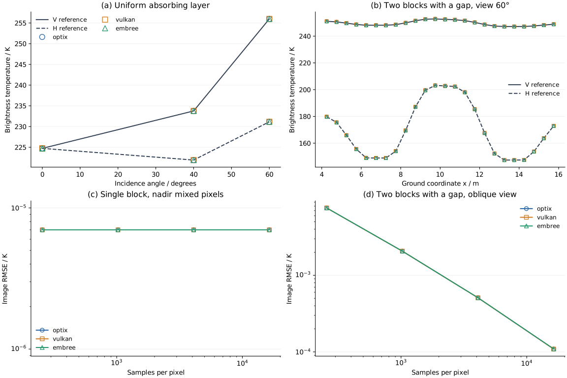
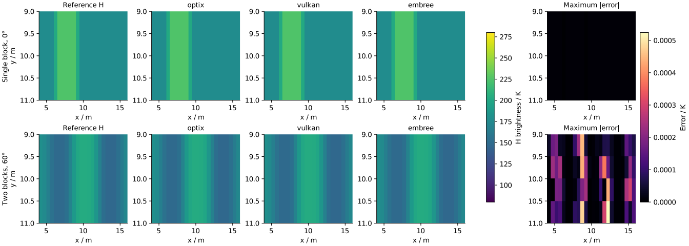
Backend	Uniform-layer maximum error / K	Finite-image RMSE / K	Maximum pixel error / K	Thermal-response closure error	Result
optix	0.00001913	0.000128	0.000524	4.230e-08	Pass
vulkan	0.00001913	0.000128	0.000524	4.230e-08	Pass
embree	0.00001913	0.000128	0.000524	4.230e-08	Pass

All 33 adopted comparisons pass across eleven added conditions and three backends; A9 now contains 75 comparisons including bare soil. Uniform-layer brightness/source limits are 0.005 K. Finite-block limits are 0.1 K for image-mean error, 0.15 K RMSE, 0.75 K maximum pixel error and 0.5 K source-mean error.

Sources must sum to output brightness. Dividing soil, vegetation and sky sources by their respective temperatures gives response coefficients whose sum must be 1; this isothermal recombination must close within 10⁻⁶.

Within-pixel positions use randomized Sobol points. Uniform layers use 1, 8 and 64 samples per pixel; finite blocks use 256, 1024, 4096 and 16384. The final two levels differ by at most 0.00011 K in image mean and 0.00048 K in image RMS, below limits of 0.05 K and 0.15 K. Single-block nadir and two-block 60° views use three different digital-shift seeds; the largest standard deviation of image-mean brightness is 4.51e-06 K.

Reproduce

Download the inputs, main script, vegetation reference and simulation script, uniform-layer mesh and finite-block mesh. Preserve the relative scripts/ and data/microwave-brightness/ directories. With LESS, NumPy and Matplotlib installed, run all comparisons:

python scripts/appendix_microwave_brightness.py

The accuracy results retain current inputs, independent references, adopted source/polarization results and sampling, seed and channel checks.